In today's post, we study the Fourier extensions of the third kind.

Intro

This series of posts looks into different strategies for interpolating non-periodic, smooth data on a uniform grid with high accuracy. For an introduction, see the first post of this series. In this post, we delve into Fourier extensions using truncated singular value decompositions. The method presented here is known as Fourier extension of the third kind as described in Boyd’s insightful paper A Comparison of Numerical Algorithms for Fourier Extension of the First, Second, and Third Kinds . SVD extensions are particularly simple and beautiful: Instead of aiming to find a periodic extension and then Fourier transform, one instead solves a linear system whose solutions are the Fourier coeffients. You may find the accompanying Python code on GitHub . The respective notebook also contains code to compute SVD extensions of arbitrary, complex functions.

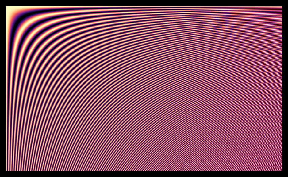
Fourier Physical Interval Collocation—Spectral Coefficients as the Unknowns (FPIC-SU)

Let \(\hat{f}(x)\), defined in \([0, \Theta]\) be the periodic extension of \(f(x)\), defined in \([0, \chi]\) where \(\Theta > \chi\). \(\hat{f}(x)\) allows for an accurate Fourier expansion as \(\hat{f}(x) = \sum_k a_k e^{\frac{2 \pi i}{\Theta} k x}\). The crucial idea of Fourier extensions of the third kind is that the coefficients \(a_k\) of the Fourier series can be obtained by solving a linear optimisation problem:

The points \(x_j\) are collocation points in the physical domain \([0, \chi]\). By solving the optimisation problem, we ensure that the mismatch between \(f(x)\) and its extension \(\hat{f}(x)\) in the physical domain is small. Does that mean that we can just invert \(M\) to solve the optimisation problem? That would be the case if \(M\) was invertible. But for a given function \(f\), one can imagine many periodic extensions that follow \(f\) in the physical domain and take different values in the extended domain. Clearly, the system is underdetermined and admits infinitely many solutions. In general, \(M\) is non-square. While \(M\) may be square-shaped if the number of collocation points \(N_{coll}\) matches the number of points of Fourier coefficients \(N\), the system is always ill-conditioned because it is close to being uninvertible. Fortunately, one can still solve the optimisation problem by computing the singular value decomposition of \(M\) and truncating small singular values before inverting \(M\).

Collocation matrix

In the following, we derive exact expressions for the above collocation matrix. Yet, solving the above complex expressions directly leads to poor results according to my numerical experiments. Instead, one should compute separate extensions for the real and imaginary parts of a complex input function. Moreover, Boyd suggests to split a general real input function \(g(x)\) into its symmetric and antisymmetric parts \(S(x) = g(x)/2 + g(-x)/2\) and \(A(x) = A(x)/2 - A(-x)/2\). The optimisation is then carried out separately for \(S\) and \(A\). The symmetric part \(S(x) \equiv f(x)\) allows for a periodic extension in terms of a cosine series whereas the antisymmetric part requires a sine series. In the following, we focus on the symmetric part, but the antisymmetric part follows analogously.

The Fourier coefficients of the cosine interpolation are the solutions of the matrix problem \(M\hat{a} = f\), where \(M_{ij} = \cos\left([j-1] \frac{\pi}{\Theta} x_i\right)\) with \(i = 1, 2, ..., N_{coll}\), \(j = 1, 2, ..., N\) and \(f_i = f(x_i)\) evaluated at \(i = 1, 2, ..., N_{coll}\). The collocation points are uniformly distributed over the positive half of the physical interval \(x\in [0, \chi]\) with \(x_i \equiv \frac{(i-1) \chi}{N_{coll} - 1}\) at the collocation indices \(i = 1, 2, ..., N_{coll}\).

The following code produces the initial plot of the collocation matrix \(M\).

import numpy as np
import matplotlib.pyplot as plt
import scipy

def get_fpic_su_matrix(N, Ncoll, theta, chi):
    x = np.zeros(Ncoll)
    M = np.zeros((Ncoll, N))
    for i in range(Ncoll):
        for j in range(N):
            #Collocation points uniformly distributed over the positive half
            #of the physical interval x in [0, chi]
            x[i]    = i * chi / (Ncoll - 1)
            M[i, j] = np.cos(j * np.pi / theta * x[i])
    return M, x

M, x  = get_fpic_su_matrix(N = 500, Ncoll = 300, theta = np.pi, chi = np.pi/2)

plt.style.use('dark_background')
fig, axs = plt.subplots(figsize=(5, 3), dpi=200)
plt.axis("off")
plt.imshow(M,  cmap="magma")
plt.tight_layout()
plt.savefig("figures/svd_W.png", bbox_inches='tight')
plt.show()

The right choice of physical and extension domain

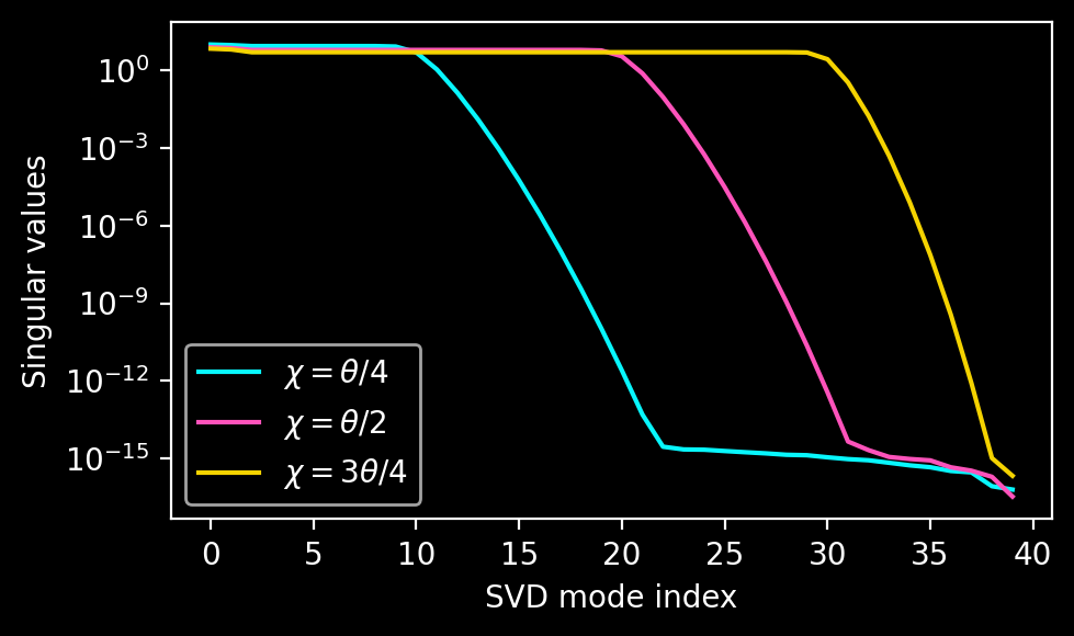
The next choice is to be made about the ideal domain sizes for the extension. The following figure shows different choices of the physical domain size \(\chi\) as a function of the extension domain size \(\Theta\). The plot shows that smaller extension domains lead to a better the conditioning of \(M\). At the same time, the resulting extensions will be less smooth and produce less accurate results. There is a trade-off between accuracy and conditioning.

The need for iterative refinement

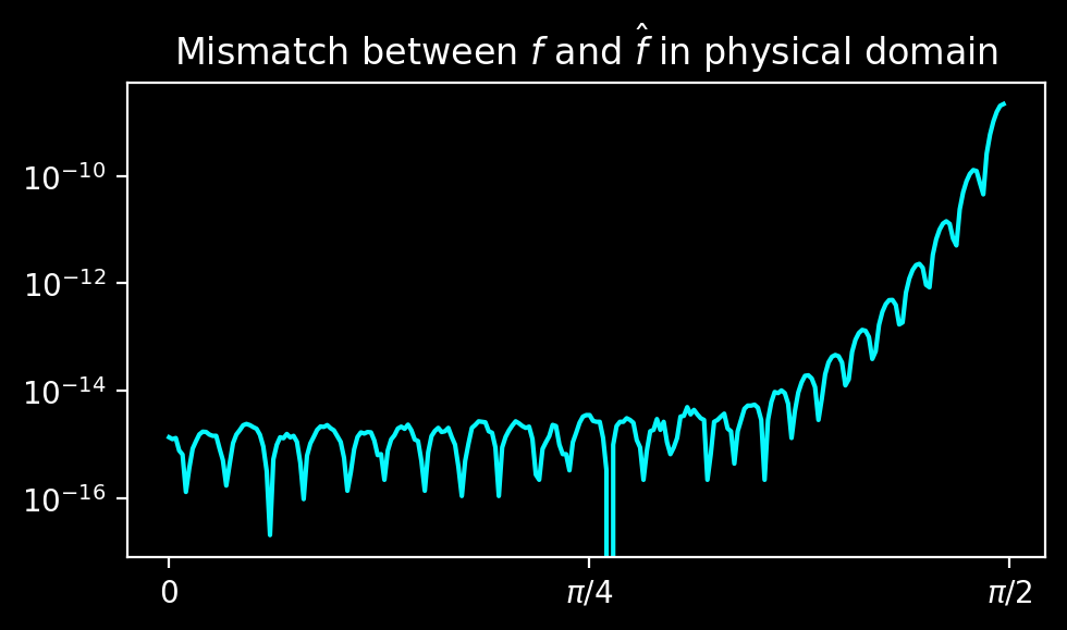
With this knowledge, we can set out to compute a periodic extension of the even function \(f(x) = x^2\) shown in the next plot. 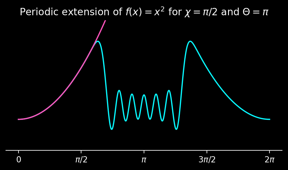The mismatch between the extension and the original function in the physical domain is good, but far from the desired machine precision. 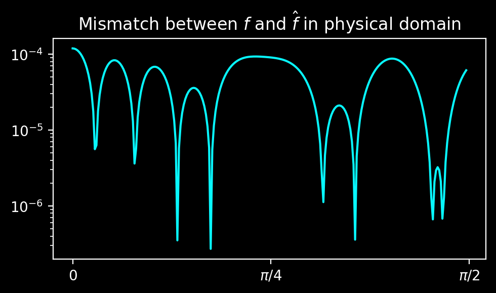As explained in Boyd’s paper, iterative refinement is another helpful trick for ill-conditioned linear systems. Applying it increases the precision of the extension drastically:

def func(x):
    return x**2

def truncated_svd_invert(M, cutoff):
    U, s, Vh = scipy.linalg.svd(M)
    sinv = np.zeros(M.T.shape)
    for i in range(np.min(M.shape)):
        if s[i] < cutoff:
            sinv[i, i] = 0
        else:
            sinv[i, i] = 1/s[i]
    return Vh.T @ sinv @ U.T

def iterative_refinement(M, Minv, f, threshold = 100, maxiter = 5):
    a       = Minv @ f
    r       = M @ a - f
    counter = 0
    while np.linalg.norm(r) > threshold * np.finfo(float).eps * np.linalg.norm(a) and counter < maxiter:
        delta    = Minv @ r
        a        = a - delta
        r        = M @ a - f
        counter += 1
    return a

def reconstruct(x, a, theta):
    rec = np.zeros(x.shape)
    for j, coeff in enumerate(a):
        rec += coeff * np.cos(np.pi / theta * j * x)
    return rec

N     = 32
Ncoll = N
theta = np.pi
chi   = theta/2
M, x  = get_fpic_su_matrix(N, Ncoll, theta, chi)
f     = func(x)
Minv  = truncated_svd_invert(M, cutoff = 1e-13)
a1    = Minv @ f
a2    = iterative_refinement(M, Minv, f, threshold = 1000, maxiter = 4)
xext  = np.linspace(0, 2 * theta, 1000)
frec1 = reconstruct(xext, a1, theta)
frec2 = reconstruct(xext, a2, theta)


for i, frec in enumerate([frec1, frec2]):
    # Plot f and extended f
    fig, axs = plt.subplots(figsize=(5 , 3), dpi=200)
    plt.title(r"Periodic extension of $f(x) = x^2$ for $\chi=\pi/2$ and $\Theta = \pi$")
    # Graphs
    plt.plot(xext, frec, label="Extension", c=colors[0])
    plt.plot(xext, func(xext), label="Original", c=colors[1])
    # Axes
    plt.ylim(np.min(frec) - 1, np.max(frec) + 1)
    plt.xticks([0, np.pi/2, np.pi, 3*np.pi/2, 2*np.pi], [0, r"$\pi/2$", r"$\pi$", r"$3\pi/2$", r"$2\pi$"])
    axs.spines['top'].set_visible(False)
    axs.spines['right'].set_visible(False)
    axs.spines['left'].set_visible(False)
    axs.get_yaxis().set_ticks([])
    # Save plot
    plt.tight_layout()
    plt.savefig(f"figures/svd_{i+1}.png", bbox_inches='tight')
    plt.legend()
    plt.show()

    # Plot error
    fig, axs = plt.subplots(figsize=(5 , 3), dpi=200)
    plt.title(r"Mismatch between $f$ and $\hat{f}$ in physical domain")
    # Physical domain
    ul = np.argwhere(xext<chi)[-1][0]
    xorg = xext[:ul]
    plt.yscale("log")
    plt.xticks([0, np.pi/4, np.pi/2], [0, r"$\pi/4$", r"$\pi/2$"])
    plt.plot(xorg, np.abs(func(xorg) - frec[:ul]), c=colors[0])
    plt.tight_layout()
    plt.savefig(f"figures/svd_{i+1}_accuracy.png", bbox_inches='tight')
    plt.show()

The need for overcollocation

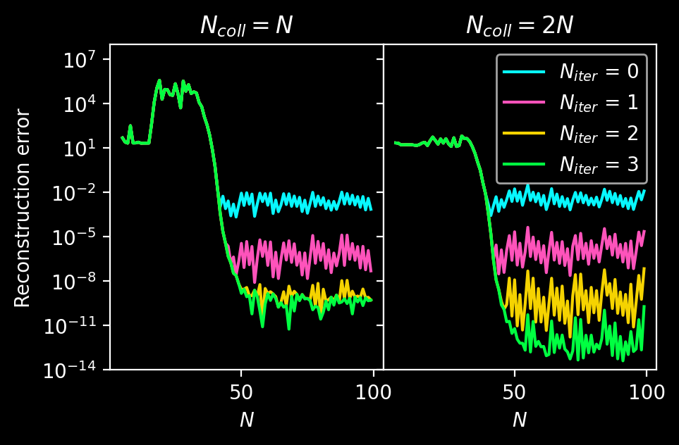
A part of the ill-conditioning of Fourier extensions stems from the fact that there are functions which are small on the collocation grid, but large in the gaps between the interpolation points. This can be remedied by having a number of collocation points \(N_{coll}\) much larger than \(N\), the number of Fourier coefficients. In this case, the scheme can detect large-amplitude oscillations of \(f\) and produce more accurate extensions. The following plot shows reconstruction errors of \(f(x) = \cos(40.5 x)\) on \([0, \pi/2]\) as a function of the number of iterations \(N_{iter}\) in the iterative refinement for different numbers \(N\) of Fourier modes in two cases: a square-matrix \(M\) where \(N_{coll} = N\) and an overcollocation case where \(N_{coll} = 2\cdot N\). The achievable accuracy in the second case is significantly higher.

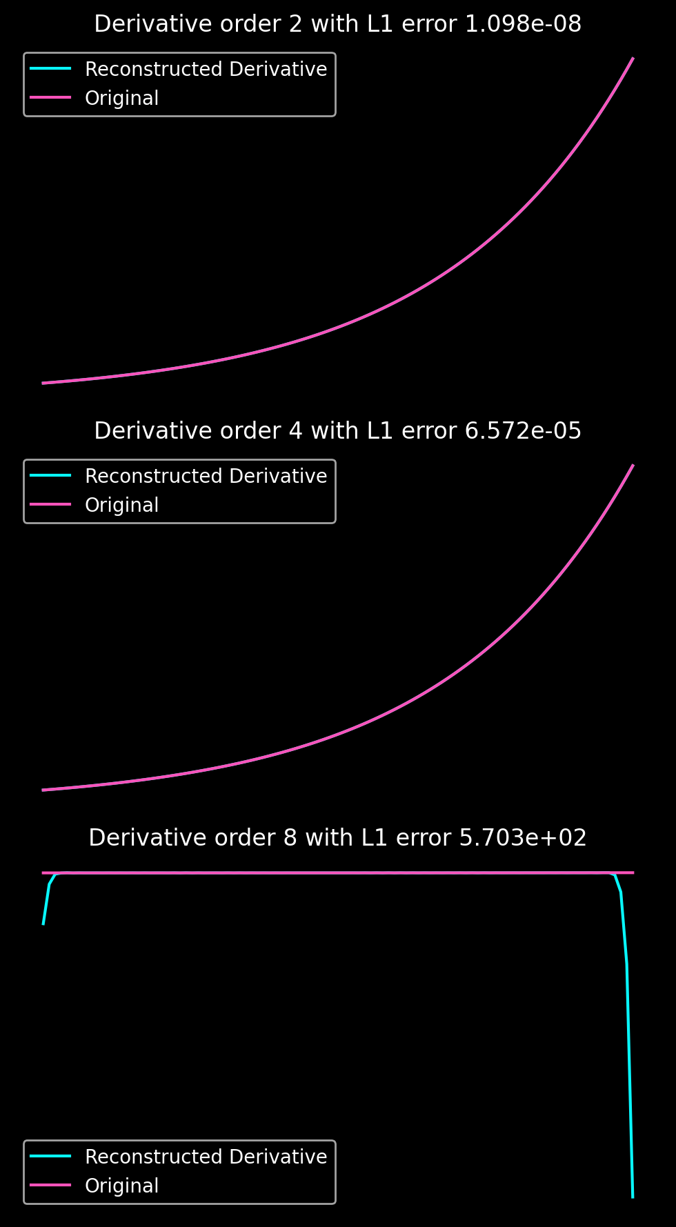
For the sake of comparability, the following plot shows the accuracy of derivatives of \(f(x) = \exp(x)\) computed using SVD extensions with \(N_{coll} = 2 N\), \(N=100\) on \([0, \chi = \pi]\) for \(N_{iter} = 10\) refinement iterations. While the accuracy is high, the ill-conditioning of the collocation matrix prevents us from accessing high-order derivatives. Note that this extension needs a generalisation of the even extension developed above. You can find the more general code at the end of the Jupyter notebook in the Github repository.

Issues

Fourier extensions of the third kind can be very accurate when overcollocation and iterative refinement are used. This accuracy comes at a price, however: A typical SVD factorisation requires \(\mathcal{O}(N^3)\) operations. The iteration refinement adds \(\mathcal{O}(2 N^2 + 2 N_{coll}^2)\) operations per iteration. The overcollocation requirement dictates that the resolution in the extension domain is lower than in the physical domain. When the number of collocation points is limited as in the case of interpolation or a PDE solver, the requirements of Fourier extensions of the third kind can be hardly met and are computationally prohibitively expensive. In addition, my own numerical experiments indicate that numerical stability of a PDE solver built with this method is an issue. Lastly, there are no analytical convergence guarantees for Fourier extensions of the third kind. Fortunately, all of these issues are resolved by Gram-Fourier extensions that we are going to look at in the last part of this series.