When Fourier fails: Subtraction
In today's post, we study ways to accurately interpolate non-periodic, smooth data on a uniform grid.
Intro
This series of posts looks into different strategies for interpolating non-periodic, smooth data on a uniform grid with high accuracy. For an introduction, see the first post of this series. In the following, we will look at subtraction methods. You may find the accompanying Python code on GitHub .
Subtraction Methods
A finite Fourier series, associated with a non-periodic function \(f\), converges very slowly, like \(\mathcal{O}(N^{-1})\) where \(N\) is the number of Fourier collocation points. One can increase this accuracy by smoothing the non-periodic function at the domain boundaries. Subtracting a known function \(F\) at the boundaries so that \(g = f - G \in C^0\) (g is continuous at the domain boundary), the associated Fourier series converges like \(\mathcal{O}(N^{-2})\). Subtraction methods estimate the function’s derivatives at the domain boundary, often employing finite difference approximations. Then, they identify a suitable set of non-periodic functions that meet the estimated boundary conditions, typically by solving a linear system. These basis functions are subtracted from the original data, leaving a smoother function conducive to an accurate Fourier transform. Moreover, the basis functions can be analytically manipulated.
Subtraction methods commonly involve subtracting either polynomials or trigonometric functions. Their accuracy hinges on the precise estimation of the data’s derivatives at the boundaries. Sköllermo used partial integration to show that if a function \(f \in C^{2p - 1}\) and \(f^{(2p)}\) is integrable, the Fourier coefficients decay as \(\propto \mathcal{O}(N^{-(2p - 1)})\). However, the maximum order of convergence is fundamentally limited by a variant of Runge’s phenomenon, as it is impossible to estimate arbitrarily high-order derivatives using polynomial stencils. In addition, high-order subtraction methods may be relatively unstable when building PDE solvers. Based on my experience with wave and fluid equations, I do not believe that PDE solvers using subtraction methods can compete with DFT solvers for periodic PDEs because they become unstable for high subtraction orders.
In the following, I will implement two subtraction methods: trigonometric and polynomial subtraction.
Trigonometric Subtraction
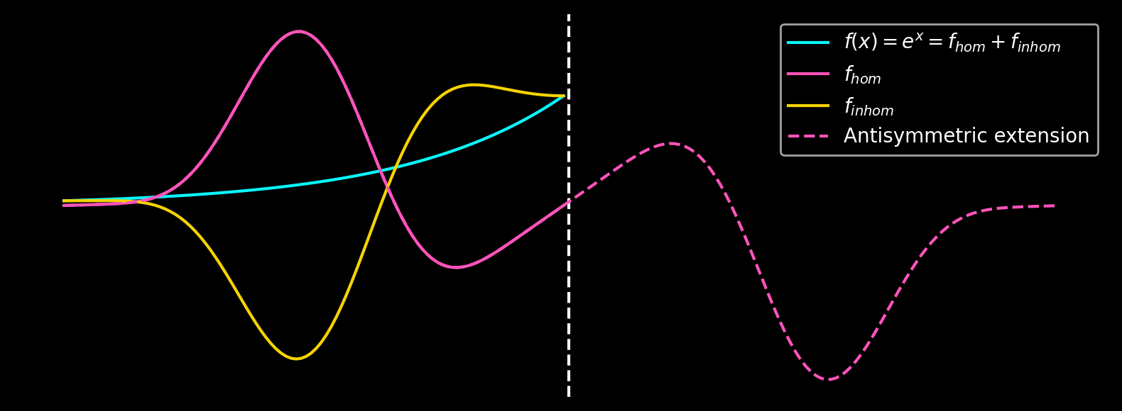
The trigonometric method, described in Matthew Green’s M.Sc. thesis Spectral Solution with a Subtraction Method to Improve Accuracy, estimates boundary derivatives using finite-difference stencils and subtracts an inhomogeneous linear combination of cosine functions, leaving a homogeneous remainder. This remainder can either be expanded using a sine transform or, less efficiently, antisymmetrically expanded into a periodic function and then manipulated using a Fourier transform. Schematically, the process looks as follows:
- Given a grid: \(0, \Delta x, ..., L - \Delta x, L\)
- Estimate even derivatives \(f^{(0)}(x_0), f^{(0)}(x_1), f^{(2)}(x_0), f^{(2)}(x_1),\)… of \(f(x)\) at \(x_0=0\) and \(x_1 = L\)
- Set them to \(0\) by subtracting suitable linear combinations of cosine functions evaluated on the discrete grid
- Define antisymmetric extension as \(\{f(x_0), ..., f(x_1), -f(x_1 - \Delta x), ..., -f(x_0 + \Delta x)\}\)
- Accurate Fourier transform of antisymmetric extension
Extension
It is useful to construct an antisymmetric extension because the \(0^{th}\) order derivatives, i.e. the function values, are known already.
Ideally, a sine transform should be used instead of the of the antisymmetric extension. It has the same analytical properties as the antisymmetric extension and is twice as fast as a DFT. The following figure demonstrates the latter process using an exponential function.
Accuracy
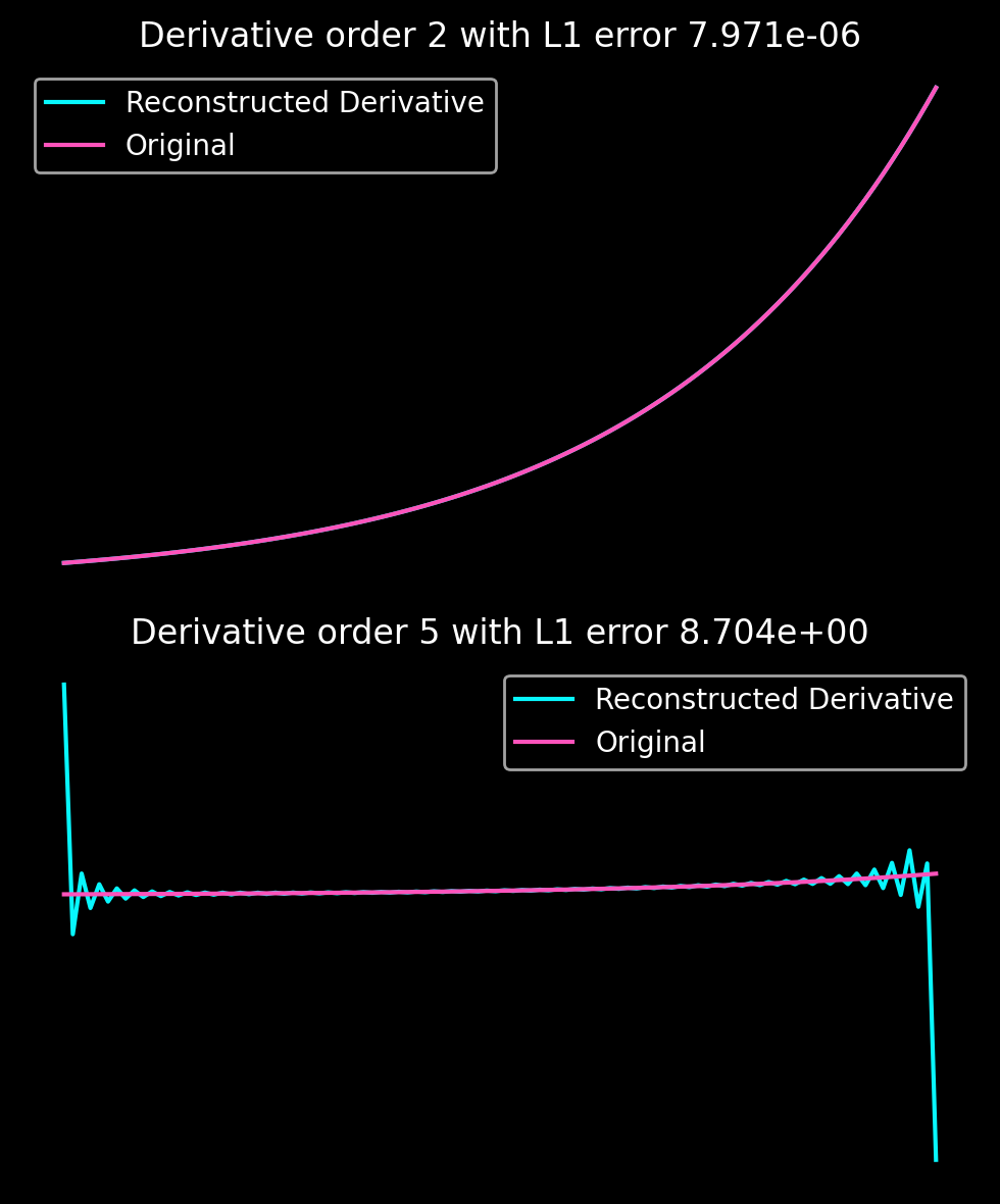
Computing derivatives by summing analytical derivatives of cosine functions with the appropriate coefficients and numerical derivatives of the Fourier transform, we see that while the first derivate can be computed very accurately, higher derivatives become less and less accurate.
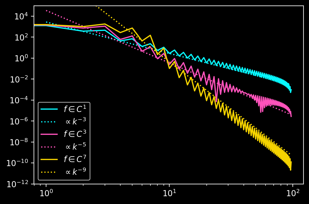
Decay of Fourier Coefficients
Finally, the decay of the Fourier coefficients can be beautifully visualised. The stability and complexity of the algorithm is determined by how many derivatives are estimated. All odd derivatives of the antisymmetric extension are continuous at the domain boundary for smooth input data. Therefore, ensuring continuity of the function at the domain boundary implies that the Fourier coefficients decay like \(\mathcal{O}(N^{-3})\), faster than without the antisymmetric extension. This can be done by subtracting a linear combination of two cosine functions such that the remainder satisfies Dirichlet boundary conditions. Every further pair of trigonometric functions subtracted increases the order of convergence by \(2\). Note that there are additional discretisation errors from the DFT and the approximation of the boundary derivatives discussed in the above references.
Polynomial Subtraction
For the polynomial subtraction, I demonstrate a slightly different approach. Instead of constructing an antisymmetric extension, I simply subtract all derivatives so that the remainder becomes periodic. The remainder can then be expanded using a DFT. In principle, one might expect antisymmetric extensions to yield higher accuracy because they achieve more continuous derivatives with the same polynomial order. However, my numerical experiments indicate that the accuracy limits of both polynomial and trigonometric subtraction because of Runge’s phenomenon are similar.
Extension
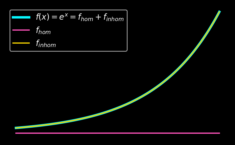
The following figure demonstrates the subtraction of a 9th-order polynomial from an exponential function. It is evident that a high-order polynomial can approximate exponential functions well, and the remainder is close to zero.
Accuracy
A suitably chosen 9th-order subtraction polynomial ensures that the homogeneous remainder is continuously differentiable four times. Accordingly, we expect order unity oscillation from the fifth derivative onwards, as confirmed by plotting the error of the reconstructed derivatives:
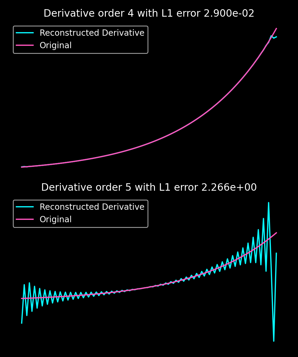
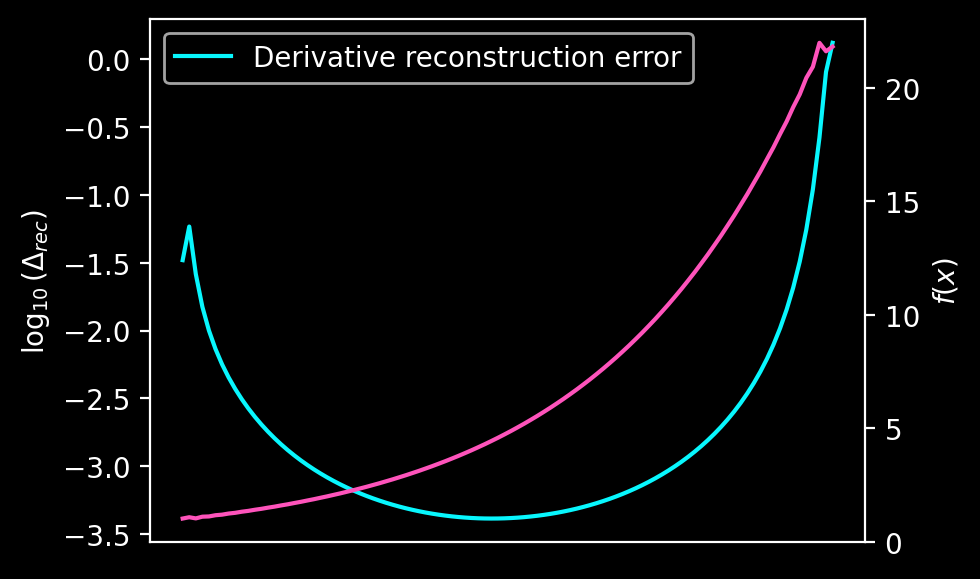
It is worth noting that, in my experience, all spectral methods acting on non-periodic data (including Chebyshev methods on Chebyshev grids) share one drawback: reconstruction errors at the domain boundaries close to the discontinuities are often orders of magnitude higher than in the domain center. This is also demonstrated in the following figure, where the logarithm of the reconstruction error is shown in blue, and the reconstructed function is in red.
Decay of Fourier Coefficients
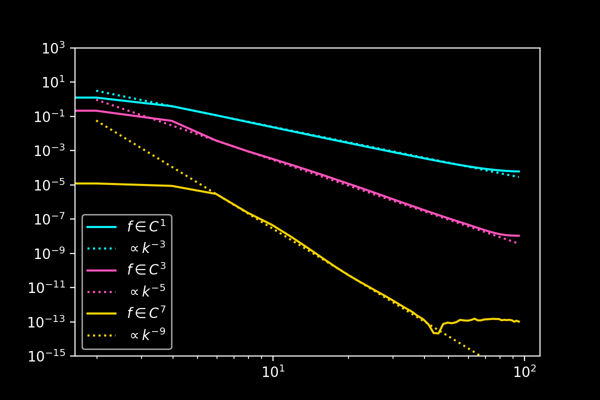
Studying the decay of the polynomial coefficients reveals that every pair of polynomials subtracted increases the order of convergence by \(1\), not by \(2\) as in the case of the antisymmetric extension. Comparing the decay of coefficients between the two methods shows that the polynomial subtraction method decays to machine precision faster than the trigonometric subtraction method despite the same order of convergence. This is one of the reasons why I do not think one of the two methods is to be preferred over the other necessarily.
Code
Code for Trigonometric Subtraction
import numpy as np
import scipy
import matplotlib.pyplot as plt

def forward_difference_matrix(order, dx):
    """
    Create a forward difference matrix of a given order and spacing.

    Args:
        order (int): The order of the matrix.
        dx (float): The spacing between points.

    Returns:
        numpy.ndarray: The forward difference matrix.
    """
    size = order
    mat = np.zeros((size, size))
    for k in range(1, size + 1):
        for j in range(1, size + 1):
            mat[j - 1, k - 1] = (j * dx) ** k / np.math.factorial(k)

    return mat

def backward_difference_matrix(order, dx):
    """
    Create a backward difference matrix of a given order and spacing.

    Args:
        order (int): The order of the matrix.
        dx (float): The spacing between points.

    Returns:
        numpy.ndarray: The backward difference matrix.
    """
    size = order
    mat = np.zeros((size, size))
    for k in range(1, size + 1):
        for j in range(1, size + 1):
            mat[j - 1, k - 1] = (-j * dx) ** k / np.math.factorial(k)

    return mat

def forward_difference_vector(order, f):
    """
    Create a forward difference vector for a given function and order.

    Args:
        order (int): The order of the difference.
        f (numpy.ndarray): The function values.

    Returns:
        numpy.ndarray: The forward difference vector.
    """
    diff = np.zeros(order)
    for j in range(1, order + 1):
        diff[j - 1] = f[j] - f[0]
    return diff

def backward_difference_vector(order, f):
    """
    Create a backward difference vector for a given function and order.

    Args:
        order (int): The order of the difference.
        f (numpy.ndarray): The function values.

    Returns:
        numpy.ndarray: The backward difference vector.
    """
    diff = np.zeros(order)
    for j in range(1, order + 1):
        diff[j - 1] = f[-1 - j] - f[-1]
    return diff

def iterative_refinement(A, b, tolerance=1e-12):
    """
    Solve a system of linear equations Ax = b using iterative refinement.

    Args:
        A (numpy.ndarray): The matrix A.
        b (numpy.ndarray): The vector b.
        tolerance (float): The tolerance for the residual error.

    Returns:
        numpy.ndarray: The solution vector x.
    """
    x = np.linalg.solve(A, b)
    residual = b - A @ x
    residual_error = np.sum(np.abs(residual))

    iteration = 0
    while residual_error > tolerance:
        correction = np.linalg.solve(A, residual)
        x += correction
        residual = b - A @ x
        residual_error = np.sum(np.abs(residual))
        iteration += 1
        if iteration > 1000:
            break

    return x

def shift_x(x):
    """
    Normalize the x values to a range of [0, 1].

    Args:
        x (numpy.ndarray): The input x values.

    Returns:
        numpy.ndarray: The normalized x values.
    """
    return (x - x[0]) / (x[-1] - x[0])

def cosine_difference_vector(order, f, Dl, Dr):
    """
    Create a cosine difference vector for a given function and order.

    Args:
        order (int): The order of the difference.
        f (numpy.ndarray): The function values.
        Dl (numpy.ndarray): The left difference values.
        Dr (numpy.ndarray): The right difference values.

    Returns:
        numpy.ndarray: The cosine difference vector.
    """
    b = np.zeros(2 * order)
    b[0] = f[0]
    b[1] = f[-1]
    #Even derivatives at left boundary
    for i in range(1, order):
        b[i * 2] = Dl[2*i-1] / (np.pi) ** (2 * i)

    #Even derivatives at right boundary
    for i in range(1, order):
        b[i * 2 + 1] = Dr[2*i-1] / (np.pi) ** (2 * i)

    return b

def cosine_difference_matrix(order):
    """
    Create a cosine difference matrix of a given order.

    Args:
        order (int): The order of the matrix.

    Returns:
        numpy.ndarray: The cosine difference matrix.
    """
    A = np.zeros((order * 2, order * 2))
    for i in range(order):
        derivative = 2 * i
        for j in range(1, 2 * order + 1):
            A[2 * i, j - 1] = j ** derivative * (-1) ** i
            A[2 * i + 1, j - 1] = j ** derivative * (-1) ** i * (-1) ** j

    return A

def reconstruct(C, x, derivative_order=0):
    """
    Reconstruct a function from its cosine series coefficients.

    Args:
        C (numpy.ndarray): The cosine series coefficients.
        x (numpy.ndarray): The x values.
        derivative_order (int): The order of the derivative to reconstruct.

    Returns:
        numpy.ndarray: The reconstructed function values.
    """
    f = np.zeros(x.shape)
    L = x[-1] - x[0]
    x_eval = shift_x(x)
    for k in range(1, len(C) + 1):
        f += C[k - 1] * np.real((1j * k * np.pi / L) ** derivative_order * np.exp(1j * k * np.pi * x_eval))

    return f

def get_shift_function(f, n_accuracy, x):
    """
    Calculate the shift function for a given function, order, and x values.

    Args:
        f (numpy.ndarray): The function values.
        n_accuracy (int): The number of even derivatives made continuous
        x (numpy.ndarray): The x values.

    Returns:
        tuple: The shift function values and the coefficients.
    """
    x_eval = shift_x(x)
    dx = x_eval[1] - x_eval[0]
    A = forward_difference_matrix(n_accuracy * 2, dx)
    b = forward_difference_vector(n_accuracy * 2, f)
    Dl = iterative_refinement(A, b)

    A = backward_difference_matrix(n_accuracy * 2, dx)
    b = backward_difference_vector(n_accuracy * 2, f)

    Dr = iterative_refinement(A, b)

    A = cosine_difference_matrix(n_accuracy + 1)
    b = cosine_difference_vector(n_accuracy + 1, f, Dl, Dr)
    C = iterative_refinement(A, b)

    shift = reconstruct(C, x_eval)
    return shift, C


def antisymmetric_extension(f):
    """
    Extend a function with its antisymmetric part.

    Args:
        f (numpy.ndarray): The function values.

    Returns:
        numpy.ndarray: The extended function values.
    """
    f_ext = np.concatenate([f, -np.flip(f)[1:-1]])
    return f_ext

def get_k(p, dx):
    """
    Calculate the k values for a given array and spacing.

    Args:
        p (numpy.ndarray): The input array.
        dx (float): The spacing between points.

    Returns:
        numpy.ndarray: The k values.
    """
    N = len(p)
    L = N * dx
    k = 2 * np.pi / L * np.arange(-N / 2, N / 2)
    return np.fft.ifftshift(k)


# Configurable parameters
N        = 100  # Size of input domain
# Accuracy of subtraction
# For a given n_accuracy, n_accuracy even derivatives are made continuous (and the function values at the boundaries are subtracted)
# Therefore, the antisymmetric extension will be in C1 + 2 * n_accuracy derivatives
# The Fourier coefficients then decay as O(3 + 2 * n_accuracy)
n_accuracy = 2

# Define the domain and the function
L = np.pi

x = np.linspace(0, L, N)
def func(x):
    return np.exp(x)
f = func(x)
dx = x[1] - x[0]

# Get the shift function and coefficients
shift, C = get_shift_function(f, n_accuracy, x)
hom      = f - shift
f_ext    = antisymmetric_extension(hom)
f_hat    = scipy.fft.fft(f_ext)

# Get the k values
k = get_k(f_hat, dx)


colors = [
    '#08F7FE',  # teal/cyan
    '#FE53BB',  # pink
    '#F5D300',  # yellow
    '#00ff41', # matrix green
]

plt.style.use('dark_background')
plt.figure(figsize=(8, 3), dpi=200)
plt.axis("off")
plt.plot(f, c = colors[0], label=r"$f(x) = e^x = f_{hom} + f_{inhom}$")
plt.plot(hom, c = colors[1], label=r"$f_{hom}$")
plt.plot(shift, c = colors[2], label=r"$f_{inhom}$")
plt.axvline(len(x), ls="dashed", c="w")
plt.plot(f_ext, c = colors[1], ls="dashed", label="Antisymmetric extension")
plt.legend()
plt.savefig("figures/subtraction_trigonometric_extension.png")
plt.show()

# Number of subplots
num_subplots = 2

# Create subplots
fig, axs = plt.subplots(num_subplots, 1,  figsize=(5 , 3* num_subplots), dpi=200)


# Loop through different subtraction orders
for i, o in enumerate([2, 5]):
    forg = func(x)
    frec = scipy.fft.ifft(f_hat * (1j * k) ** o).real[:N]  # Use only the first N elements (the original domain)
    reco = reconstruct(C, x, derivative_order = o)
    sumo = frec + reco

    axs[i].spines['top'].set_visible(False)
    axs[i].spines['right'].set_visible(False)
    axs[i].spines['bottom'].set_visible(False)
    axs[i].spines['left'].set_visible(False)
    axs[i].get_xaxis().set_ticks([])
    axs[i].get_yaxis().set_ticks([])

    # Plot the sum and the original function in subplots
    axs[i].set_title(f"Derivative order {o} with L1 error {np.mean(np.abs(sumo - forg)):3.3e}")
    axs[i].plot(x, sumo, label="Reconstructed Derivative", c = colors[0])
    axs[i].plot(x, forg, label="Original", c = colors[1])
    axs[i].legend()

# Adjust layout
fig.savefig("figures/subtraction_trigonometric_accuracy.png")
Code for Polynomial Subtraction
import numpy as np
import matplotlib.pyplot as plt
import scipy.fft
import scipy.interpolate

# Constants for finite difference modes
MODE_FORWARD = 0
MODE_CENTERED = 1
MODE_BACKWARD = 2
MODE_CUSTOM = 3

# Max derivative order allowed
MAX_DERIVATIVE_ORDER = 30

# Finite difference stencils for forward, backward, and centered modes
fstencils = []
bstencils = []
cstencils = []


def compute_fd_coefficients(derivative_order, n_accuracy, mode, stencil=None):
    """
    Compute finite difference coefficients for given derivative order and n_accuracy.

    Args:
        derivative_order (int): The order of the derivative.
        n_accuracy (int): The n_accuracy of the approximation.
        mode (int): The mode of finite difference (forward, backward, centered, custom).
        stencil (np.array): The points used for the finite difference.

    Returns:
        tuple: A tuple containing the stencil and the coefficients.
    """
    stencil_length = derivative_order + n_accuracy

    if mode == MODE_FORWARD:
        stencil = np.arange(0, stencil_length)
    elif mode == MODE_BACKWARD:
        stencil = np.arange(-stencil_length + 1, 1)
    elif mode == MODE_CENTERED:
        if n_accuracy % 2 != 0:
            raise ValueError("Centered stencils available only with even n_accuracy orders")
        if (stencil_length % 2 == 0) and stencil_length >= 4:
            stencil_length -= 1
        half_stencil_length = int((stencil_length - 1) / 2)
        stencil = np.arange(-half_stencil_length, half_stencil_length + 1)
    elif mode == MODE_CUSTOM:
        if stencil is None:
            raise ValueError("Custom stencil needed in MODE_CUSTOM")
        stencil_length = len(stencil)
        if derivative_order >= stencil_length:
            raise ValueError("Derivative order must be smaller than stencil length")

    A = np.zeros((stencil_length, stencil_length))
    b = np.zeros(stencil_length)

    for i in range(stencil_length):
        A[i, :] = stencil ** i
    b[derivative_order] = np.math.factorial(derivative_order)

    coefficients = np.linalg.solve(A, b)
    return stencil, coefficients


# Populate the finite difference stencils for forward, backward, and centered modes
for i in range(MAX_DERIVATIVE_ORDER):
    N_MAX = i + 2
    fstencils_at_order_i = []
    bstencils_at_order_i = []
    cstencils_at_order_i = []
    for order in range(1, N_MAX):
        c = compute_fd_coefficients(order, N_MAX - order + ((N_MAX - order) % 2 != 0), MODE_CENTERED)
        f = compute_fd_coefficients(order, N_MAX - order, MODE_FORWARD)
        b = compute_fd_coefficients(order, N_MAX - order, MODE_BACKWARD)
        fstencils_at_order_i.append(f)
        bstencils_at_order_i.append(b)
        cstencils_at_order_i.append(c)
    fstencils.append(fstencils_at_order_i)
    bstencils.append(bstencils_at_order_i)
    cstencils.append(cstencils_at_order_i)


def compute_derivative(f, j, dx, stencil, derivative_order=1):
    """
    Compute the derivative of a function at a point.

    Args:
        f (np.array): The function values.
        j (int): The index of the point.
        dx (float): The spacing between points.
        stencil (tuple): The stencil and coefficients for finite differences.
        derivative_order (int): The order of the derivative.

    Returns:
        float: The derivative of the function at point j.
    """
    shifts, coeff = stencil
    f_dx = sum(f[j + shift] * coeff[i] for i, shift in enumerate(shifts))
    return f_dx / dx ** derivative_order


def get_polynomial_shift_function(f, n_accuracy, x):
    """
    Compute the polynomial shift function to fulfill Dirichlet boundary conditions.

    Args:
        f (np.array): The function values.
        n_accuracy(int): The number of derivatives made continuous: f - shift will be in the set of continuous, order-times differentiable functions C^order(x)
        x (np.array): The domain of the function.

    Returns:
        tuple: The polynomial shift function and the interpolating polynomial.
    """
    dx = x[1] - x[0]
    x0, x1 = x[0], x[-1]
    f0, f1 = f[0], f[-1]

    N_columns    = 1 + n_accuracy
    fd_f_stencil = fstencils[n_accuracy - 1]
    fd_b_stencil = bstencils[n_accuracy - 1]

    B = np.zeros((N_columns, len(f)), f.dtype)

    bc_l = [(i + 1, compute_derivative(f, 0, dx, fd_f_stencil[i], i + 1)) for i in range(n_accuracy)]
    bc_r = [(i + 1, compute_derivative(f, -1, dx, fd_b_stencil[i], i + 1)) for i in range(n_accuracy)]

    bc = (bc_l, bc_r)

    poly = scipy.interpolate.make_interp_spline([x0, x1], [f0, f1], k=2 * n_accuracy + 1, bc_type=bc, axis=0)

    for i in range(n_accuracy + 1):
        B[i] = poly(x, i * 2)

    return B[:, :len(x)], poly


# Configurable parameters
N        = 100  # Size of input domain
# Accuracy of the subtraction, this leads to a polynomial of order 2*n_accuracy + 1 being subtracted from the original function
n_accuracy = 4

# Define the domain and the function
L = np.pi
x = np.linspace(0, L, N)


def func(x):
    """Function to compute e^x."""
    return np.exp(x)


f = func(x)
dx = x[1] - x[0]

# Create shift function such that f - B fulfills Dirichlet boundary conditions
shift, polynomial_func = get_polynomial_shift_function(f = f, n_accuracy=n_accuracy, x = x)
f_ext = f - shift[0]
f_hat = scipy.fft.fft(f_ext)

# Function to get k values
k = get_k(f_hat, dx)

colors = [
    '#08F7FE',  # teal/cyan
    '#FE53BB',  # pink
    '#F5D300',  # yellow
    '#00ff41',  # matrix green
]

plt.style.use('dark_background')
plt.figure(figsize=(5, 3), dpi=200)
plt.axis("off")
plt.plot(f, c=colors[0], lw=3, label=r"$f(x) = e^x = f_{hom} + f_{inhom}$")
plt.plot(f_ext, c=colors[1], label=r"$f_{hom}$")
plt.plot(shift[0], c=colors[2], label=r"$f_{inhom}$")
plt.legend()
plt.savefig("figures/subtraction_polynomial_extension.png")
plt.show()