When Fourier fails: Mollifiers
In today's post, we introduce mollifiers at the example of the local Fourier basis method. You may find the accompanying Python code on GitHub.
Intro
This series of posts looks into different strategies for interpolating non-periodic, smooth data on a uniform grid with high accuracy. For an introduction, see the first post of this series. In this post, we delve into the benefits of mollifiers, which involve convolutions of non-periodic data with smooth bell functions around discontinuities to ensure continuity. The method presented here is presented as Fourier extension of the second kind in Boyd’s insightful paper A Comparison of Numerical Algorithms for Fourier Extension of the First, Second, and Third Kinds. It also features in the paper Spectral multidomain technique with Local Fourier Basis by Israeli et al. who use it to build PDE solvers.
Mollifiers
Mollifiers involve convolving non-periodic functions with suitable smooth bell functions in position space to smooth out discontinuities. Unlike filters, mollifiers require knowledge of the discontinuity’s location, making them less effective in certain applications. Similar to filters, convolution with a mollifier results in information loss, making them less effective than methods that utilize more information about the function to achieve periodicity.
The mollifier we are going to is the bell function \(B(x)\):
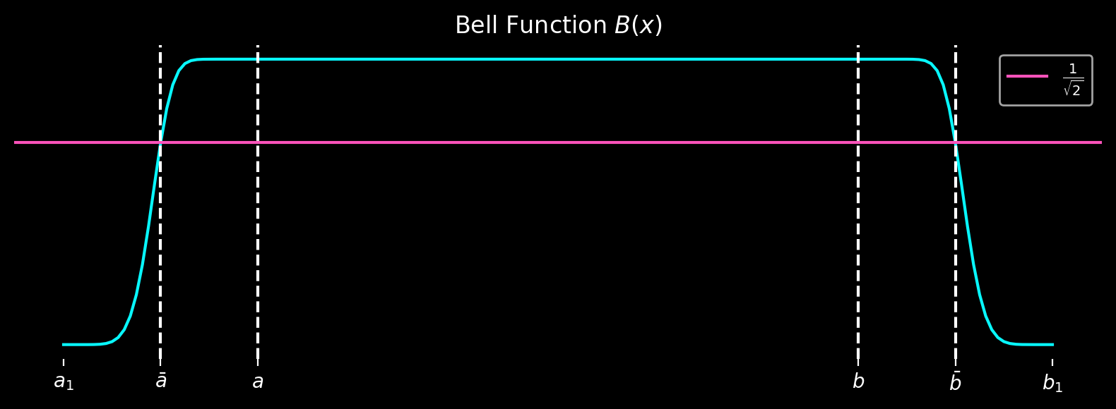 It is the identity function in the domain \([a, b]\) and smoothly decays to zero in the boundary regions \([a_1, a]\) and \([b, b_1]\). Moreover, it assumes the value \(\frac{1}{\sqrt{2}}\) at the points \(\bar{a}\) and \(\bar{b}\).
Antisymmetric extension
One could naively multiply the bell function \(B(x)\) with the input function \(f(x)\) to obtain a periodic function. However, as Boyd’s paper suggests, higher accuracy can be achieved through a folding operation that optimally utilizes the boundary zone.
\[F(x) = B(x)f(x) - B(2\hat{a} - x) f(2\hat{a} - x) - B(2\hat{b} - x) f(2\hat{b} - x)\]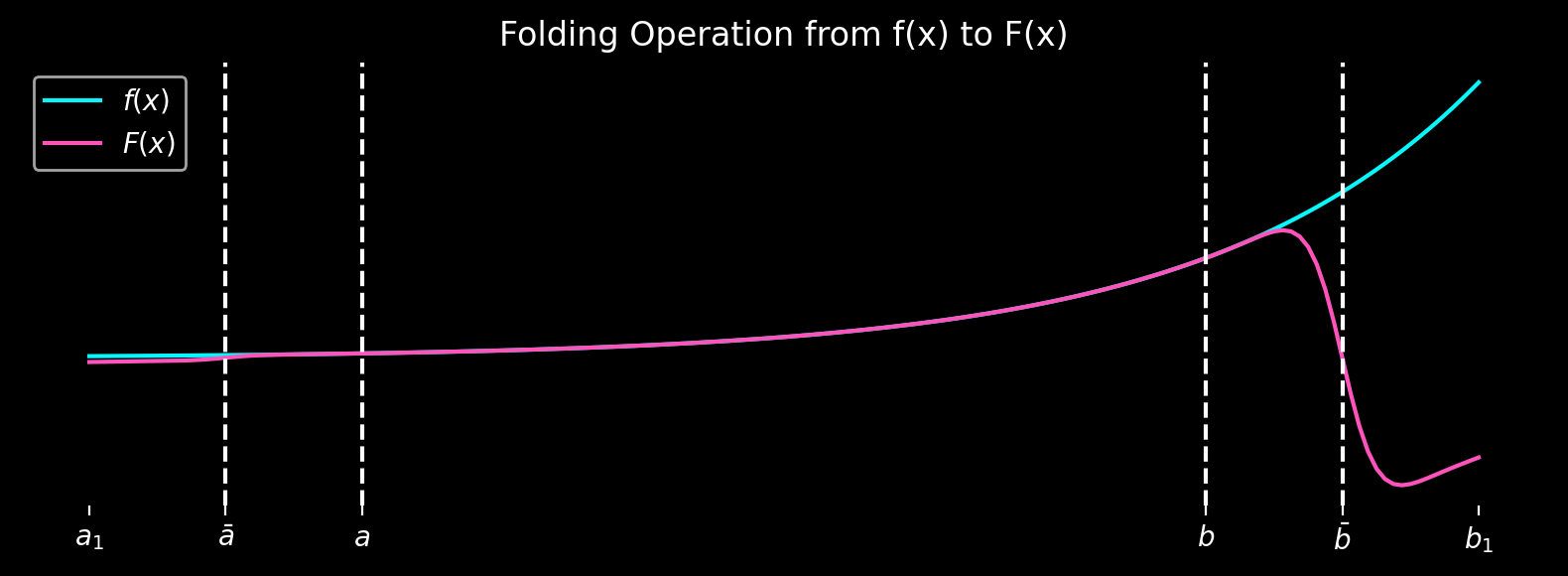
\(F(x)\) can be antisymmetrically extended to produce a periodic function, where the original unmodified function \(f(x)\) resides in the shaded domain shown below.
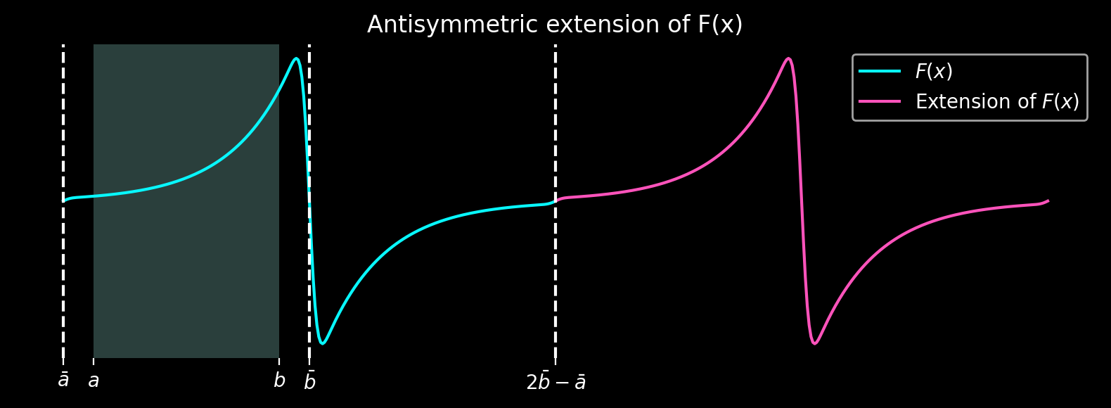
It is important to note that in this process, the boundary regions \([a_1, a]\) and \([b, b_1]\) are discarded. The larger these regions are, the higher the accuracy of the periodic extension.
Accuracy
For a domain of size \(N=100\) and additional ghost boundaries of size \(N_{gh} = 32\) we obtain the following accuracies for the derivatives of \(f(x) = \exp(x)\) in \([0, \pi]\).
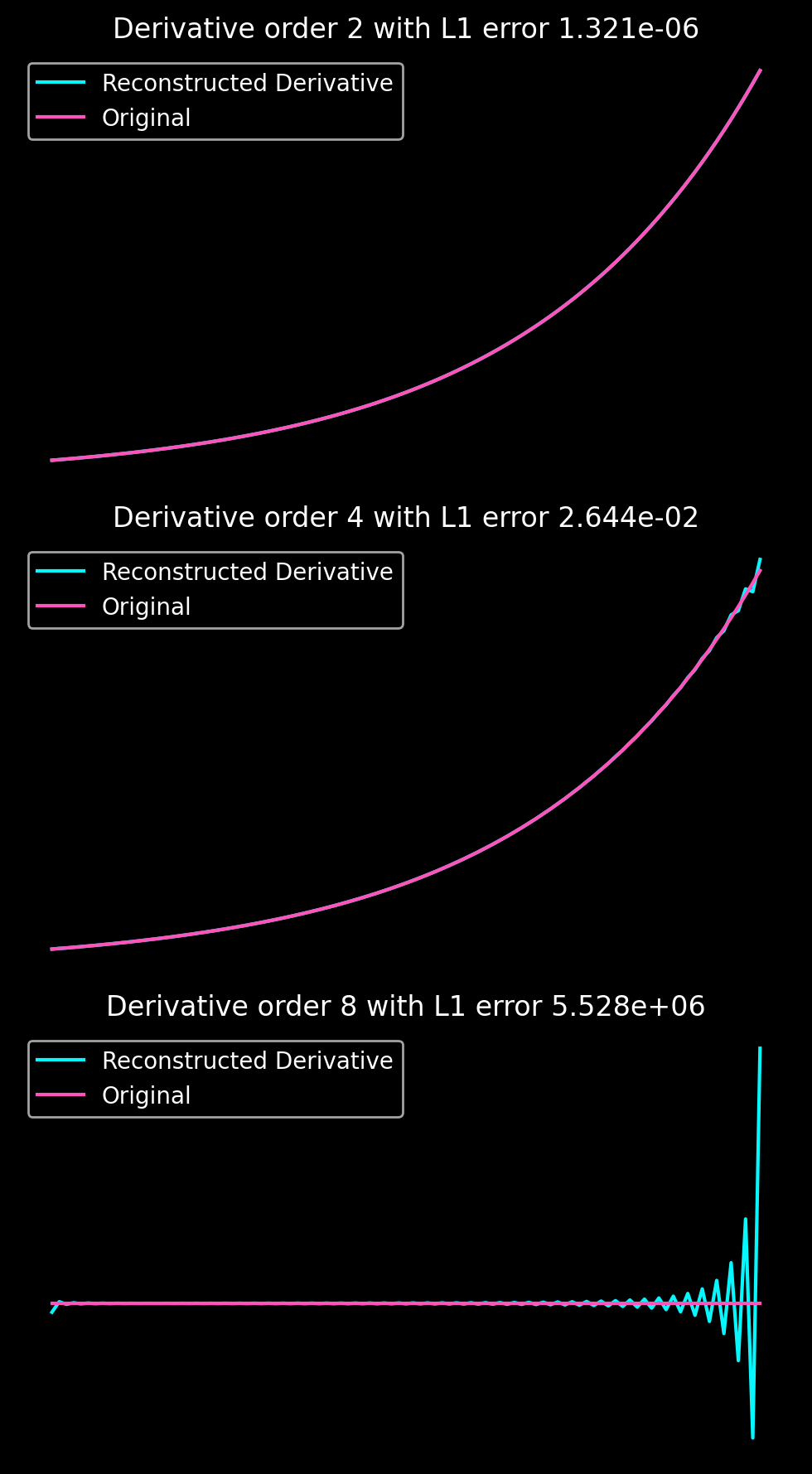
While the accuracy is acceptable, it falls short of expectations when sacrificing more than one-third of the input data for obtaining a periodic extension. However, mollifiers offer the advantage of not requiring the solution of linear systems of equations, making them computationally efficient. They can be a viable option for large domains where having a ghost boundary of a few dozen points is feasible.
Code
import numpy as np
import scipy
import matplotlib.pyplot as plt

L                 = np.pi
N                 = 100
dx                = L/(N - 1)
ghostBoundary     = 32
x                 = np.arange(-ghostBoundary, N + ghostBoundary) * dx

def theta(x, eps):
    return np.pi/4 * ( 1 + np.sin( np.pi/2 * np.sin( np.pi/2 * np.sin ( np.pi/2 * x / eps ))))

def sfunc(x, eps):
    return np.sin(theta(x, eps))

def cfunc(x, eps):
    return np.cos(theta(x, eps))

def bfunc(x, a1, a, b1, b):
    B = np.zeros(x.shape)
    eps  = (b1 - b) / 2

    c = (x >= a1) * (x <= a)
    B[ c ] = sfunc( x[c] + eps, eps )
    c = (x >= a) *  (x <= b)
    B[ c ] = 1
    c = (x > b) * (x <= b1)
    B[ c ] = cfunc( x[c] - eps - b, eps)
    return B

a1 = - ghostBoundary * dx
a  =   0
b  =   L
b1 = + ghostBoundary * dx  + L
ab = (a + a1)/2
bb = (b + b1)/2

colors = [
    '#08F7FE',  # teal/cyan
    '#FE53BB',  # pink
    '#F5D300',  # yellow
    '#00ff41', # matrix green
]

plt.style.use('dark_background')
fig, ax = plt.subplots(figsize=(8, 3), dpi=200)
ax.spines['top'].set_visible(False)
ax.spines['right'].set_visible(False)
ax.spines['bottom'].set_visible(False)
ax.spines['left'].set_visible(False)
ax.get_yaxis().set_ticks([])
plt.title(r"Bell Function $B(x)$")
plt.plot(x, bfunc(x, a1, a, b1, b), c = colors[0])
plt.axhline(1/np.sqrt(2), label=r"$\frac{1}{\sqrt{2}}$", c = colors[1])
plt.axvline(a, ls="dashed")
plt.axvline(b, ls="dashed")
plt.axvline(ab, ls="dashed")
plt.axvline(bb, ls="dashed")
plt.xticks(ticks=[a1, ab, a, b, bb, b1], labels=[r"$a_1$", r"$\bar{a}$", r"$a$", r"$b$", r"$\bar{b}$", r"$b_1$", ])
plt.legend()
plt.tight_layout()
plt.savefig("figures/lfb_bell.png", bbox_inches='tight')
plt.show()

def func(x):
    return np.exp(x)

f = func(x)
B = bfunc(x, a1, a, b1, b)

def folding(x, func, bfunc):
    return bfunc(x, a1, a, b1, b) * func(x) - bfunc(2 * ab - x, a1, a, b1, b) * func(2 * ab - x) - bfunc(2 * bb - x, a1, a, b1, b) * func(2 * bb - x)

def fhat(f, B):
    return f * B - np.flip(np.roll(B * f, -ghostBoundary)) - np.roll(B * f, ghostBoundary)


fig, ax = plt.subplots(figsize=(8, 3), dpi=200)
ax.spines['top'].set_visible(False)
ax.spines['right'].set_visible(False)
ax.spines['bottom'].set_visible(False)
ax.spines['left'].set_visible(False)
ax.get_yaxis().set_ticks([])
plt.title(r"Folding Operation from f(x) to F(x)")
plt.plot(x, func(x), label=r"$f(x)$", c = colors[0])
plt.plot(x, folding(x, func, bfunc), label=r"$F(x)$", c = colors[1])
plt.axvline(a, ls="dashed")
plt.axvline(b, ls="dashed")
plt.axvline(ab, ls="dashed")
plt.axvline(bb, ls="dashed")
plt.xticks(ticks=[a1, ab, a, b, bb, b1], labels=[r"$a_1$", r"$\bar{a}$", r"$a$", r"$b$", r"$\bar{b}$", r"$b_1$", ])
plt.legend()
plt.tight_layout()
plt.savefig("figures/lfb_symmetric.png", bbox_inches='tight')
plt.show()


def Ffunc(x, func, bfunc):
    Nh  = N + ghostBoundary
    Nl  =  Nh * 2 - 1
    xl  = np.arange(-ghostBoundary/2, N + ghostBoundary/2) * dx
    # Exclude left boundary since it agrees with right boundary of xl
    xh = (xl + bb - ab)[1:]
    X  = np.arange(-ghostBoundary/2, Nl-ghostBoundary/2) * dx
    F  = np.zeros(Nl)
    F[:Nh] = folding(         xl, func, bfunc)
    F[Nh:] = -folding(2 * bb - xh, func, bfunc)
    return X, F

X, F = Ffunc(x, func, bfunc)

L = 2*bb - 2*ab

fig, ax = plt.subplots(figsize=(8, 3), dpi=200)
ax.spines['top'].set_visible(False)
ax.spines['right'].set_visible(False)
ax.spines['bottom'].set_visible(False)
ax.spines['left'].set_visible(False)
ax.get_yaxis().set_ticks([])
plt.title(r"Antisymmetric extension of F(x)")
plt.plot(X, F, label=r"$F(x)$", c = colors[0])
plt.plot(X + L, F, label=r"Extension of $F(x)$", c = colors[1])
plt.axvspan(a, b, alpha = 0.3)
plt.axvline(ab, ls="dashed")
plt.axvline(bb, ls="dashed")
plt.axvline(2 * bb - ab, ls="dashed")
plt.xticks(ticks=[a, b, ab, bb, 2 * bb - ab, ], labels=[r"$a$", r"$b$", r"$\bar{a}$", r"$\bar{b}$", r"$2 \bar{b} - \bar{a}$", ])
plt.legend()
plt.tight_layout()
plt.savefig("figures/lfb_extension.png", bbox_inches='tight')
plt.show()


# Number of subplots
num_subplots = 3

# Create subplots
fig, axs = plt.subplots(num_subplots, 1,  figsize=(5 , 3* num_subplots), dpi=200)


def get_k(p, dx):
    """
    Calculate the k values for a given array and spacing.

    Args:
        p (numpy.ndarray): The input array.
        dx (float): The spacing between points.

    Returns:
        numpy.ndarray: The k values.
    """
    N = len(p)
    L = N * dx
    k = 2 * np.pi / L * np.arange(-N / 2, N / 2)
    return np.fft.ifftshift(k)


f_hat = scipy.fft.fft(F[:-1]) # F[0] = F[-1] by construction

# Get the k values
k = get_k(f_hat, dx)

s = (X[:-1]>=a) * (X[:-1]<b) # select physical domain and discard ghost boundaries

xorg = X[:-1][s]
forg = func(xorg)

# Loop through different subtraction orders
for i, o in enumerate([2, 4, 8]):
    frec = scipy.fft.ifft(f_hat * (1j * k) ** o).real  # Use only the first N elements (the original domain)
    frec = frec[s]
    axs[i].spines['top'].set_visible(False)
    axs[i].spines['right'].set_visible(False)
    axs[i].spines['bottom'].set_visible(False)
    axs[i].spines['left'].set_visible(False)
    axs[i].get_xaxis().set_ticks([])
    axs[i].get_yaxis().set_ticks([])

    # Plot the sum and the original function in subplots
    axs[i].set_title(f"Derivative order {o} with L1 error {np.mean(np.abs(frec - forg)):3.3e}")
    axs[i].plot(xorg, frec, label="Reconstructed Derivative", c = colors[0])
    axs[i].plot(xorg, forg, label="Original", c = colors[1])
    axs[i].legend()

# Adjust layout
fig.tight_layout()
fig.savefig("figures/lfb_accuracy.png", bbox_inches='tight')