In today's post, we study the truncated Inverse Polynomial Reconstruction method.

Intro

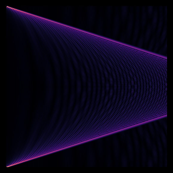
This series of posts looks into different strategies for interpolating non-periodic, smooth data on a uniform grid with high accuracy. For an introduction, see the first post of this series. In this post, we delve into a very interesting topic: Inverse Polynomial Reconstruction (IPR). The method presented here is described in Jung’s and Shizgal’s paper On the numerical convergence with the inverse polynomial reconstruction method for the resolution of the Gibbs phenomenon . The logic of this method is as follows: We compute the Fourier extension of a non-periodic function and then change to a basis with better convergence properties. The result is a highly accurate reconstruction of the original function in a polynomial basis on a uniform grid. This result is surprising since direct polynomial expansion leads to the Runge instability. The idea to restore convergence of the Fourier series in a different basis has been pioneered by Gottlieb et al. using Gegenbauer polynomials. However, there is an important difference between the Gegenbauer and IPR methods. While the Gegenbauer method achieve stability by projection of the Fourier basis onto a polynomial basis spanning a smaller subspace, the IPR method computes an invertible change-of-base matrix between arbitrary functional bases. Convergence is independent of the polynomial basis used. Stability is remedied by the truncation suggested by Jung et al. which is effectively the truncation the Gegenbauer method started with. I only present IPR theory since it supersedes Gegenbauer methods according my understanding. You may find the accompanying Python code on GitHub . Below you can catch a glimpse of the change-of-basis matrix we are going to derive in the following.

Change-of-basis matrix

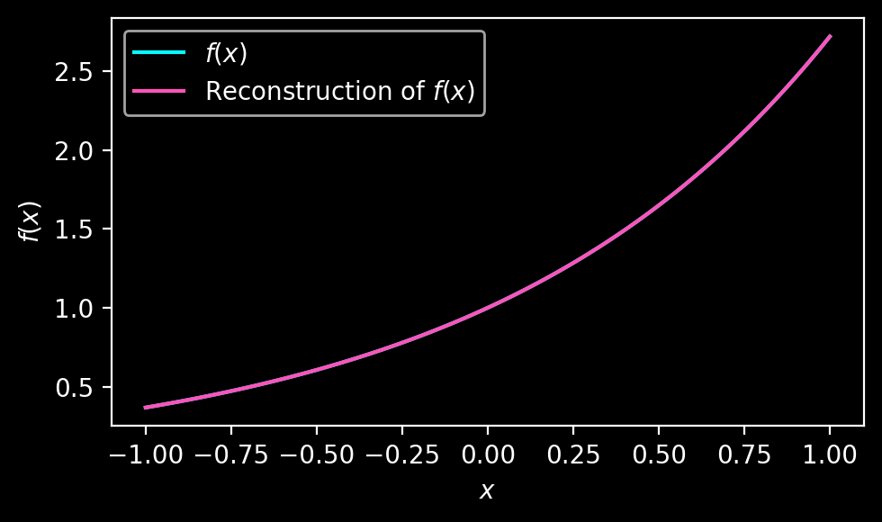
Let us study the Fourier transform of \(f(x) = \exp(x)\) on \([-1, 1]\).

import numpy as np
import scipy
import matplotlib.pyplot as plt
N   = 100
x   = np.linspace(-1, 1, N)
f   = np.exp(x)
f_k = scipy.fft.fft(f)

The Fourier coefficients \(\hat{f}_k\) of a discrete Fourier series \(f_N(x) = \sum_{k=-N}^{N} \hat{f}_k \exp(i k \pi x)\) can be defined via the Fourier inner product

In this expression, the Fourier transform of \(f(x)\) can be understood as \(\hat{f}_k\) being the projection of \(f(x)\) onto the \(k\)-th basis element of the Fourier basis. Let us introduce a different basis set \(\{\phi_l(x), l = 0, ..., m\}\) and choose \(\phi_l\) to be the Chebyshev polynomials. We can compute the change-of-basis matrix \(W\) from the Chebyshev basis to the Fourier basis using the Fourier transform as

\(W_{kl} = (\phi_l(x), \exp(i k \pi x))_F = \frac{1}{2} \int_{-1}^1 \phi_l(x) \exp(-i\pi x k) \mathrm{d}x\)

W = np.zeros((N, N), dtype=complex)

for l in range(N):
    W[:, l] = scipy.fft.fft(scipy.special.chebyt(l)(x))

Assuming that \(W\) is a non-singular matrix, we can invert it, multiply it with \(f_k\) and reconstruct \(f(x)\) by summing the Chebyshev polynomials

W_inv = np.linalg.inv(W)
g     = W_inv @ f_k

f_rec = np.poly1d([])
for l, coeff in enumerate(g):
    f_rec += coeff * scipy.special.chebyt(l)

fig, axs = plt.subplots(figsize=(5 , 3), dpi=200)
plt.style.use('dark_background')
plt.plot(x, f, label = r"$f(x)$", c = '#08F7FE')
plt.plot(x, f_rec(x), label = r"Reconstruction of $f(x)$", c = '#FE53BB')

The result looks as follows: 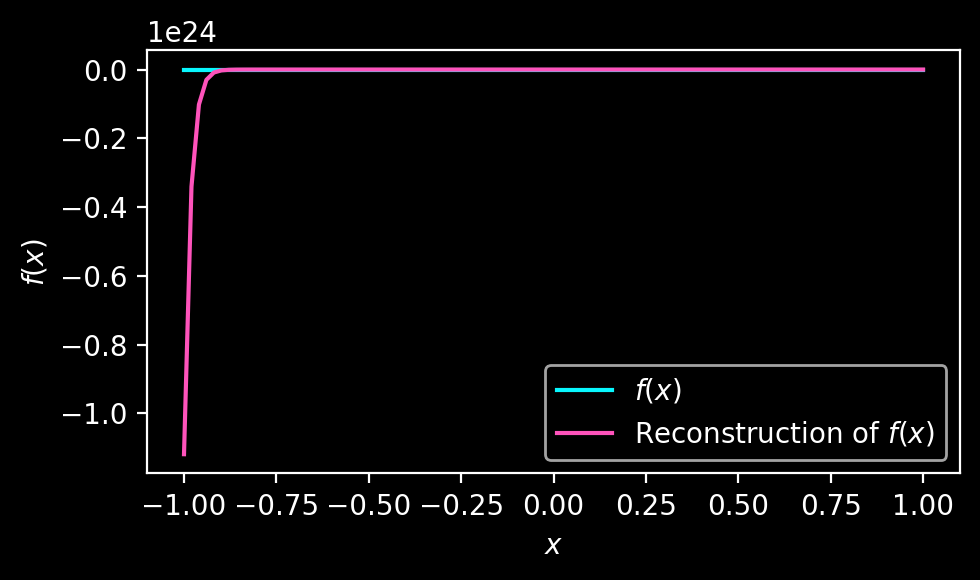What went wrong? The reconstruction is clearly divergent and the problem lies in the conditioning of \(W\), as is confirmed by plotting its singular values: 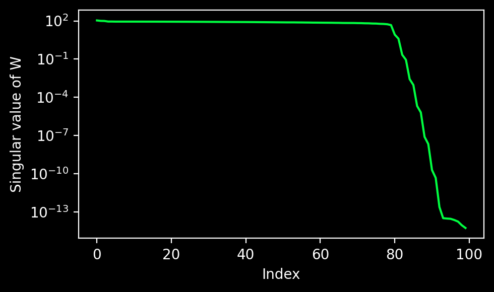Its condition number in this case is \(\mathrm{cond}(W) = 10^{16}\). Fortunately for us, Jung’s paper proposes a solution: A projection to a polynomial subspace performed via Gaussian elimination with a truncation:

# LU decomposition with pivot
pivot, L, U = scipy.linalg.lu(W, permute_l=False)

# forward substitution to solve for L x y = f_k
y = np.zeros(f_k.size, dtype=complex)
for m, b in enumerate((pivot.T @ f_k).flatten()):
    y[m] = b
    # skip for loop if m == 0
    if m:
        for n in range(m):
            y[m] -= y[n] * L[m,n]
    y[m] /= L[m, m]

# truncation for IPR
c = np.abs(y) < 1000 * np.finfo(float).eps
y[c] = 0

# backward substitution to solve for y = U x
g = np.zeros(f_k.size, dtype=complex)
lastidx = f_k.size - 1  # last index
for midx in range(f_k.size):
    m = f_k.size - 1 - midx  # backwards index
    g[m] = y[m]
    if midx:
        for nidx in range(midx):
            n = f_k.size - 1  - nidx
            g[m] -= g[n] * U[m,n]
    g[m] /= U[m, m]


f_rec = np.poly1d([])
for l, coeff in enumerate(g):
    f_rec += coeff * scipy.special.chebyt(l)

fig, axs = plt.subplots(figsize=(5 , 3), dpi=200)
plt.style.use('dark_background')
plt.plot(x, f, label = r"$f(x)$", c = '#08F7FE')
plt.plot(x, f_rec(x), label = r"Reconstruction of $f(x)$", c = '#FE53BB')
plt.xlabel(r"$x$")
plt.ylabel(r"$f(x)$")
plt.legend()
plt.tight_layout()
plt.savefig("figures/ipr_success.png", bbox_inches='tight')
plt.show()

The truncated reconstruction beautifully converges. The only downside of this method is that the truncation threshold needs to be empirically determined and should be set high enough to ensure stability.

Accuracy

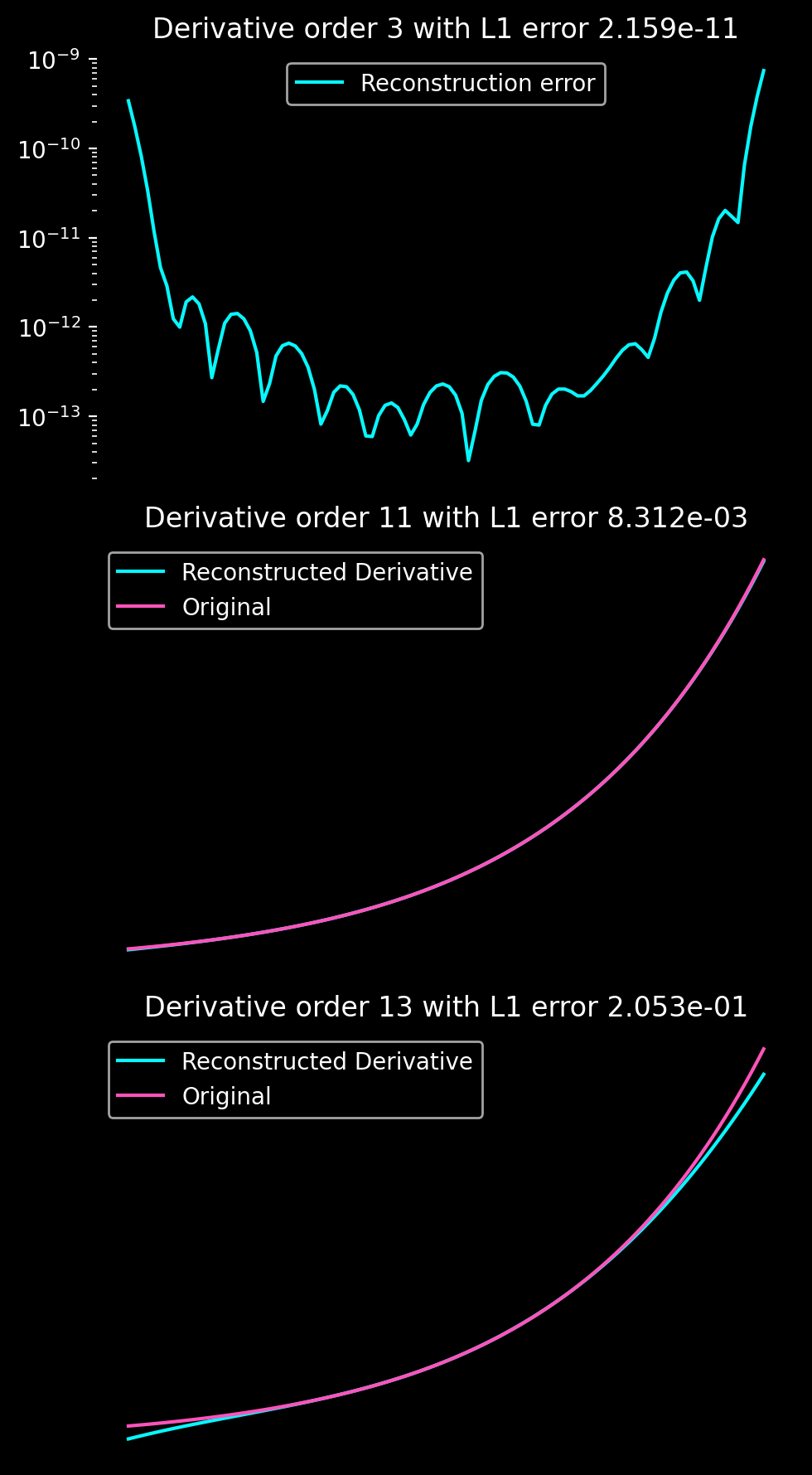
The accuracy of the truncated IPR is very high and can reach machine precision. The first plot in the series demonstrates that despite a high precision, the IPR shares a feature that I have observed in all spectral reconstructions of non-periodic data: The errors close to the discontinuity at the domain boundaries is orders of magnitude higher than in the domain center. Whatever the approach, having a ghost boundary that can be discarded helps to achieve high accuracy. The second plot shows that even an \(11\)th order derivative can be calculated within \(0.1\)% error. From my experience, the IPR has very good convergence properties for large enough \(N\). However, for low-resolution data, the error of the reconstruction is unbounded which makes the IPR algorithm unsuitable for the interpolation of low-resolution data with high accuracy.