When Fourier fails: Gram-Fourier extensions
In today's post, we study the Gram-Fourier extensions. They are a cross between SVD and polynomial expansions and offer high accuracy and stability at the asymptotic cost of a single Fourier transform. You may find the accompanying Python code on GitHub.
Intro
This series of posts looks into different strategies for interpolating non-periodic, smooth data on a uniform grid with high accuracy. For an introduction, see the first post of this series. In this post, we study Gram-Fourier extensions. This method was first described in Lyon’s PhD thesis High-order unconditionally-stable FC-AD PDE solvers for general domains .
This method combines the accuracy of SVD extensions with the computational advantages of polynomial expansions.
The merits of Gram-Fourier extensions
In the previous post, we looked at SVD extensions: Periodic extensions obtained through solving a least-squares optimisation problem. They can be highly accurate, but are computationally expensive and require many collocation points for good results. The Gram-Fourier extension method remedies these drawbacks. Instead of computing SVD extensions of an interpolant at runtime, one precomputes SVD extensions of a set of polynomial basis functions, so-called Gram polynomials. The interpolant is expanded in terms of this polynomial basis set at the domain boundaries. But instead of summing the original polynomials, one then sums the precomputed periodic extensions of the polynomials and obtains a periodic function. In other words, one precomputes a change-of-basis from a polynomial basis to a periodic basis. This has several advantages: Firstly, the SVD extension of an analytically known function can be arbitrarily accurate because it can use arbitrarily many collocation points and arbitrarily high precision. Secondly, the polynomial expansion is only carried out at the interpolant’s boundaries. Since the change-of-basis is precomputed, the Gram-Fourier extension operation has constant computational cost compared to \(\mathcal{O}(N^3)\) for a standard SVD extension. The fact that the interpolant is only expanded at the boundaries means that the extension is oblivious to what the interpolant looks like away from the domain boundary. This limits the accuracy of Gram-Fourier extensions since the extension cannot be arbitrarily smooth at the domain boundary. A boundary domain containing \(N_{boundary}\) points supports a polynomial of order \(N_{boundary} - 1\). This means that one can estimate at most \(N_{boundary} - 1\) derivatives. Hence, the extension generally has \(N_{boundary}-2\) continuous derivatives. As a result, the Fourier coefficients of a Gram-Fourier extension should at most decay like \(\mathcal{O}(k^{-N_{boundary}+1})\).
Gram Polynomials
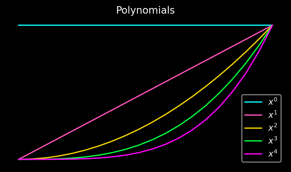
In the first step towards Gram-Fourier extensions, we start with a set of \(N\) polynomials on \(N\) points defined on the left and right boundary of the physical domain.
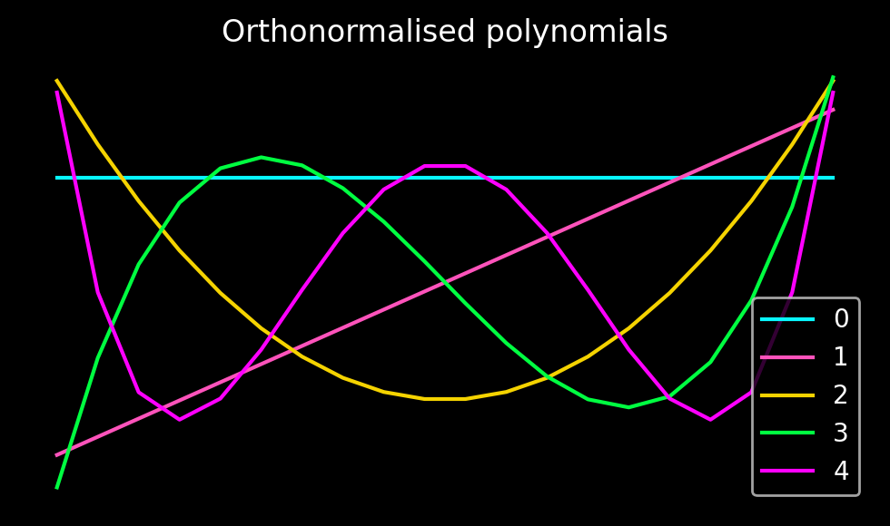
 In order to expand the interpolant in terms of these polynomials, we use the Gram-Schmidt orthogonalisation algorithm to obtain an orthonormal basis set. Since this is a one-off computation, we carry it out in high precision using Python’s mpmath library. Alternatively, all of the following computations could be carried out symbolically.
SVD Extensions
For an introduction to SVD extensions, please see the previous post in this series. In the following, we compute suitable SVD extensions of the orthonormal basis set derived in the previous section. But first, we need to make a few choices regarding the parameters of the SVD extension.
Firstly, we choose the size of the boundary domain \(n_{\Delta}\). It determines the maximum polynomial order that can live on the boundary and therefore the accuracy of the scheme. Secondly, we choose the maximum polynomial order \(m \leq n_{\Delta}\) for the boundary. Thirdly, we choose the number of collocation points \(\Lambda\) and the number of points in the extension domain \(n_D\). We have already learnt that \(\Lambda > n_D\), that is, overcollocation improves the quality of SVD extensions. Since we work in arbitrary precision, we do not need to truncate the singular values of the SVD and also do not require iterative refinement. Furthermore, we can directly solve the complex optimisation problem without a split into symmetric and antisymmetric parts. At the same time, there is an additional complication because we compute two independent extensions for the left and right domain boundary: How to stitch them together? Lyon proposes to compute an even and an odd extensions respectively using only a number of \(g\) even and odd wave vectors. By taking linear combinations of the two, one obtains extensions that smoothly decay to zero. These extensions can be stitched together to obtain a global periodic extension.
In the following, I use \(m = n_{\Delta} = 5\), \(\Lambda = 150\), \(n_D = 26\) and \(g=63\), in agreement with the parameter suggestions in Lyon’s thesis. Depending on your application, you may choose different parameters.
The following plot shows the even and odd extensions \(f_{even}\) and \(f_{odd}\) (blue graphs on the left and right) alongside the Gram polynomials (pink) of order \(0\) to \(4\) (top to bottom). The white, vertical, dashed line at \(x = \Delta\) denotes the symmetrix axis of the even and odd extensions: \(f_{even}(x) = f_{even}(x+\Delta)\) and \(f_{odd}(x) = -f_{odd}(x + \Delta)\).
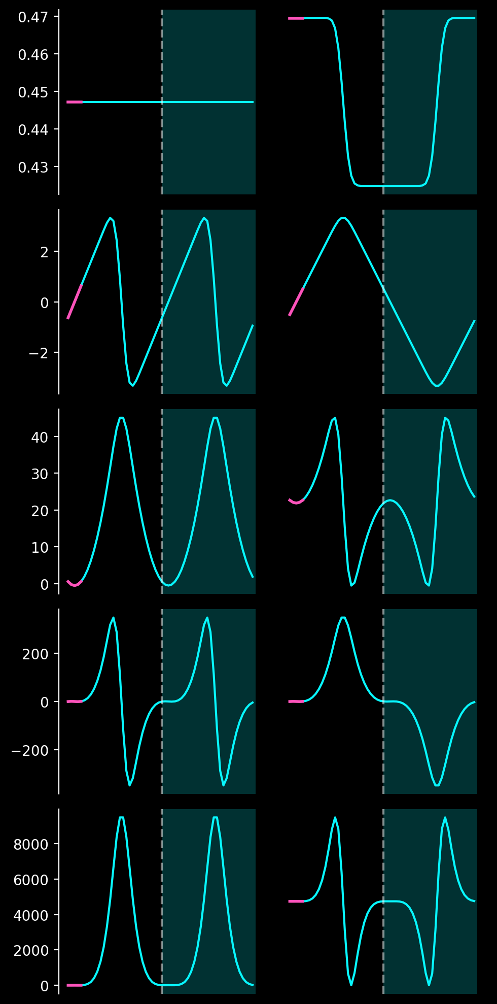
The SVD extensions so obtained describe the Gram polynomials in the physical domain very well. One can reliably achieve a maximum approximation error below any desired value on the entire physical domain.
Gram-Fourier extension
Finally, let us take a look at the function \(f(x) = \exp(x)\) on \([0, \pi]\) and compute its Gram-Fourier extension for \(N=32\). We project the function \(f\) in the left and right boundary domains onto polynomials of orders \(0\) to \(4\) to obtain \(a_{left}\) and \(a_{right}\). In the second step, we use these coefficients to compute linear combinations of the even and odd extensions that smoothly decay to zero.
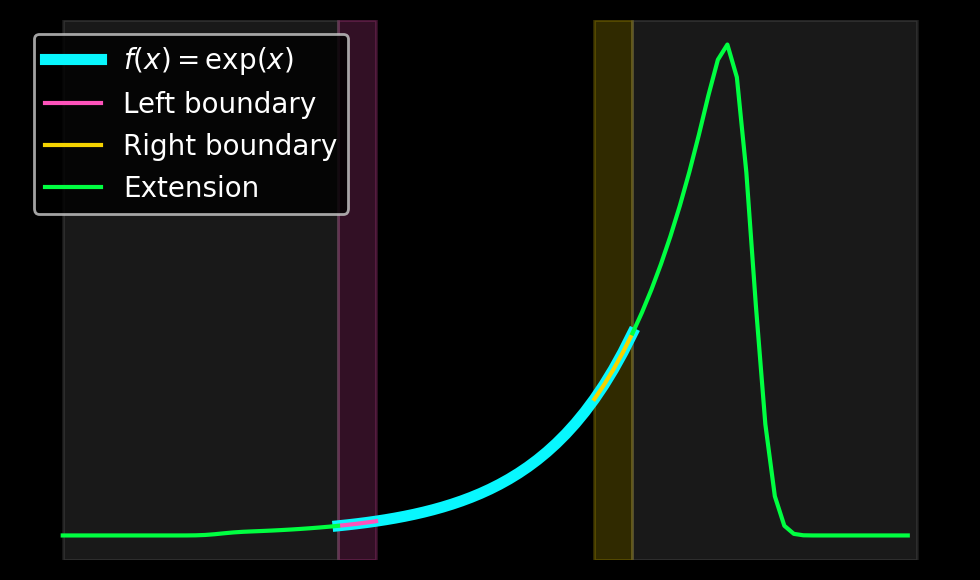
Ignoring the parts where the extension is zero, one obtains the following plot:
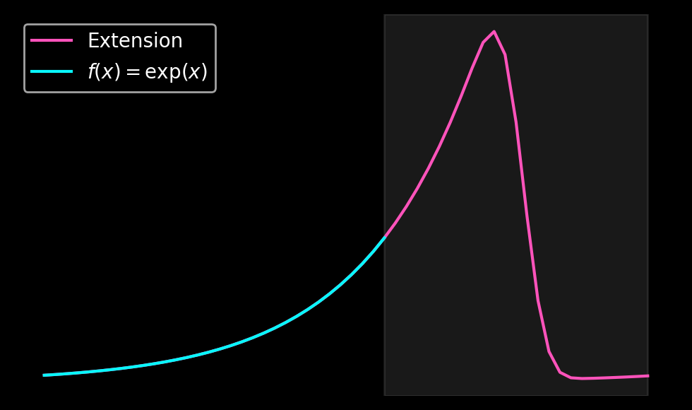
This extension only requires two matrix multiplications by \(m \times m\) matrices to obtain the coefficients \(a_{left}\) and \(a_{right}\) as well as a linear combination of the precomputed extensions.
def func(x):
    return np.exp(x)
L   = np.pi
N   = 32
dx  = L/N
x   = np.arange(0, N) * dx
f   = func(x)

# Interpolant at boundaries
f_left   = f[:nDelta]
f_right  = f[-nDelta:]

# Project interpolant at boundaries onto Gram polynomials
a_left   = Pl_numpy @ f_left
a_right  = Pr_numpy @ f_right

# Project interpolant at boundaries onto Gram polynomials
f_left_rec  = a_left @ Pl_numpy
f_right_rec = a_right @ Pr_numpy

f_zero_left  = a_left/2  @ F_even_numpy - a_left/2  @ F_odd_numpy
f_zero_right = a_right/2 @ F_even_numpy + a_right/2 @ F_odd_numpy


f_ext_left  = f_zero_left[:nd+nDelta-1]
f_ext_right = f_zero_right[nDelta-1:-nd+2]

fig, axs = plt.subplots(figsize=(5, 3), dpi=200)

plt.axis("off")
plt.plot(x, f)
plt.plot(x[ :nDelta], f_left_rec)
plt.axvspan(0, x[nDelta-1], color=colors[1], alpha=0.2)
plt.plot(x[-nDelta:], f_right_rec)
plt.axvspan(x[-nDelta], x[-1], color=colors[2], alpha=0.2)

plt.plot(np.arange(-len(f_ext_left) + 1, 1) * dx, f_ext_left)
plt.plot(np.arange(N-1, N - 1 + len(f_ext_right)) * dx, f_ext_right)
plt.axvspan((-len(f_ext_left) + 1) * dx, 0, color="white", alpha=0.1)
plt.axvspan((N-1) * dx, (N - 1 + len(f_ext_right)) * dx, color="white", alpha=0.1)

plt.tight_layout()
plt.savefig("figures/gramfe_zero_extension.png", bbox_inches='tight')
plt.show()


fmatch = (a_left + a_right)/2 @ F_even_numpy + (a_right - a_left)/2 @ F_odd_numpy

f_periodic = np.concatenate([f, fmatch[nDelta:nDelta + nd - 2]])

fig, axs = plt.subplots(figsize=(5, 3), dpi=200)
plt.axis("off")
plt.plot(np.arange(len(f_periodic)) * dx, f_periodic, c=colors[1], label="Extension")
plt.plot(x, f, c=colors[0], label=r"$f(x) = \exp(x)$")
plt.axvspan((N - 1) * dx, (len(f_periodic) - 1) * dx, color="white", alpha=0.1)
plt.legend()
plt.tight_layout()
plt.savefig("figures/gramfe_extension.png", bbox_inches='tight')
plt.show()
Accuracy
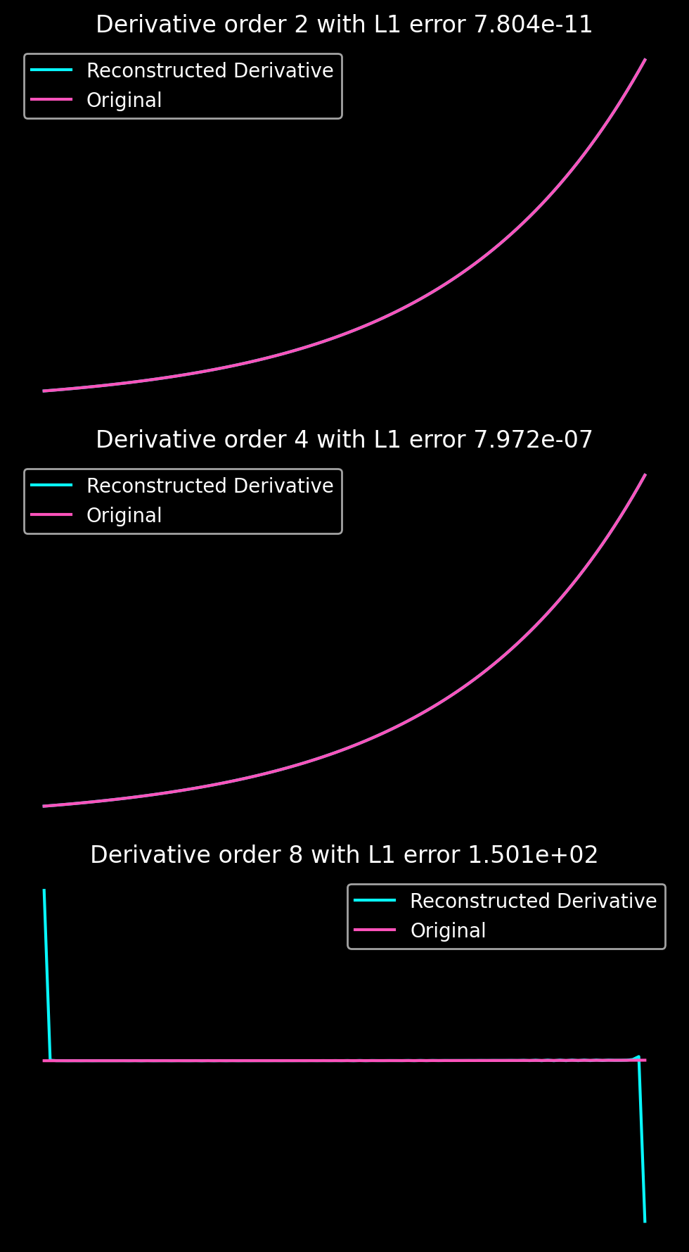
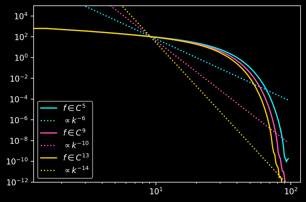
The following two plots show the reconstruction errors for derivatives using the Gram-Fourier extension for the same parameters as above with the exception of \(m = n_{\Delta} = 14\) as well as the decay of the Fourier coefficients for different values of \(m = n_{\Delta}\).
Note that the decay of the Fourier coefficients is very different from what I would have naively expected based on the smoothness of the extension at the boundary. So, please just ignore the legend. Instead, the behaviour of the Fourier coefficients seems to be dominated by the extension domain.
Conclusion
This concludes the series of posts on non-periodic interpolation. Out of all the methods presented, the Gram-Fourier extension is the most versatile. It is fast, accurate and stable. Once the extension tables are computed, it allows for an easy and fast implementation using existing matrix multplication and FFT libraries on CPUs and GPUs.
Code
The code accompanying this post is lengthy. I recommend you take a look at the Jupyter notebook in the Github repository.
import matplotlib.pyplot as plt
import numpy as np
import scipy
from mpmath import *

mp.dps = 64
eps = 1e-64

import matplotlib as mpl

plt.style.use('dark_background')

# Define your custom colors
colors = [
    '#08F7FE',  # teal/cyan
    '#FE53BB',  # pink
    '#F5D300',  # yellow
    '#00ff41',  # matrix green
    '#FF00FF',  # magenta
    '#FFA500',  # orange
    '#00FFFF',  # cyan
]

# Set the custom color cycle
mpl.rcParams['axes.prop_cycle'] = mpl.cycler(color=colors)

class GramSchmidt:
    def __init__(self, x, m):
        self.x = x
        self.m = m
        self.A = mp.zeros(m, len(x))
        #Linear map for polynomial scalar product
        for i in range(m):
            for j in range(len(x)):
                #Polynomial basis {1, x, x^2, x^3, x^4, ..., x^m}
                self.A[i, j] = x[j]**i

        #Write basis vector as columns of matrix V
        self.V = mp.eye(m)

        self.U = self.modified_gram_schmidt_algorithm(self.V)

    def evaluate_basis(self, x, basis_element_index):
        #Linear map for polynomial scalar product
        A = mp.zeros(self.m, len(x))
        for i in range(self.m):
            for j in range(len(x)):
                #Polynomial basis {1, x, x^2, x^3, x^4, ..., x^m}
                A[i, j] = x[j]**i
        ei = self.U[:, basis_element_index].T * A

        return ei

    def scalar_product(self, u, v):
        return mp.fsum((u.T * self.A) * (v.T * self.A).T)

    def project_u_onto_v(self, u, v):
        a1 = self.scalar_product(v, u)
        a2 = self.scalar_product(u, u)
        return a1/a2 * u

    def norm(self, u):
        return mp.sqrt(self.scalar_product(u, u))

    def modified_gram_schmidt_algorithm(self, V):
        n, k = V.rows, V.cols
        U    = V.copy()
        U[:, 0] = V[:, 0] / self.norm(V[:, 0])

        for i in range(1, k):
            for j in range(i, k):
                U[:, j] = U[:, j] - self.project_u_onto_v(U[:, i - 1], U[:, j])


            U[:, i] = U[:, i] / self.norm(U[:, i])
        return U

    def project_f_onto_basis(self, f):
        coeffs = mp.matrix(1, self.m)

        for i in range(self.m):
            basis = (self.U[:, i].T * self.A)
            coeffs[0, i] = mp.fsum(f * basis.T)


        return coeffs

    def reconstruct_f(self, coeffs, x = None):
        if x == None:
            A = self.A
        else:
            A = mp.zeros(self.m, len(x))
            for i in range(self.m):
                for j in range(len(x)):
                    #Polynomial basis {1, x, x^2, x^3, x^4, ..., x^m}
                    self.A[i] = x[j]**i

        frec = mp.matrix(1, A.cols)
        for i in range(self.m):
            frec += coeffs[0, i] * (self.U[:, i].T * A)
        return frec

    def plot_polynomials(self):
        m = self.m
        u_ij = mp.zeros(m)

        fig, axs = plt.subplots(figsize=(5, 3), dpi=200)
        plt.title(f"Polynomials")
        plt.axis("off")
        for i in range(m):
            plt.plot(x, self.V[:, i].T * self.A, label=f"$x^{i}$")
        plt.legend()
        plt.tight_layout()
        plt.savefig("figures/gramfe_polynomials.png", bbox_inches='tight')
        plt.show()

        fig, axs = plt.subplots(figsize=(5, 3), dpi=200)
        plt.title(f"Orthonormalised polynomials")
        plt.axis("off")
        for i in range(m):
            plt.plot(self.x, self.U[:, i].T * self.A, label=f"{i}")
        plt.legend()
        plt.tight_layout()
        plt.savefig("figures/gramfe_orthonormal_polynomials.png", bbox_inches='tight')
        plt.show()

        print("The orthonormalised polynomials and their scalar products")
        for i in range(m):
            for j in range(m):
                u_ij[i, j] = self.scalar_product(self.U[:, i], self.U[:, j])
            print(f"i = {i} u_ij = {u_ij[i, :]}")

x = mp.linspace(0, 1, 20)
gs = GramSchmidt(x, 5)
gs.plot_polynomials()

M_ALL_K  = 0
M_EVEN_K = 1
M_ODD_K  = 2


def get_wave_vectors(g, mode = M_ALL_K):
    if g % 2 == 0:
        k = np.arange(-int(-g/2) + 1, int(g/2) + 1)
    else:
        k = np.arange(-int((g-1)/2), int((g-1)/2) + 1)

    if mode == M_EVEN_K:
        k = k[k % 2 == 0]
    elif mode == M_ODD_K:
        k = k[k % 2 == 1]

    return k * mp.mpf(1)

def get_grid(Delta, Lambda):
    dxeval = Delta/(Lambda - 1)
    xeval  = mp.matrix(1, Lambda)
    for i in range(Lambda):
        xeval[0, i] = 1 - Delta + i * dxeval
    return xeval

def get_svd_extension_matrix(g, Lambda, Delta, d, mode):
    ks = get_wave_vectors(g, mode)
    x  = get_grid(Delta, Lambda)
    M  = mp.matrix(Lambda, len(ks))
    for i in range(Lambda):
        for j, k in enumerate(ks):
            M[i, j] = mp.exp(1j * k * np.pi / (d + Delta) * x[0, i])
    return M

def invert_svd_extension_matrix(M, cutoff):
    U, s, Vh = mp.svd(M)
    sinv = mp.diag(s)
    r = M.cols
    if M.rows < M.cols:
        r = M.rows
    for i in range(r):
        if s[i] < cutoff:
            sinv[i, i] = 0
        else:
            sinv[i, i] = 1/s[i]

    Vht = Vh.transpose_conj()
    Ut  = U.transpose_conj()
    f1  = sinv * Ut
    f2  = Vht * f1
    return  f2

def reconstruct_svd_extension(x, a, g, Lambda, Delta, d, mode):
    ks = get_wave_vectors(g, mode)
    rec = mp.matrix(1, len(x))
    for j, coeff in enumerate(a):
        for i in range(len(x)):
            rec[i] += coeff * mp.exp(1j * ks[j] * np.pi / (d + Delta) * x[i])
    return rec


def iterative_refinement(M, Minv, f, threshold = 100, maxiter = 1000):
    a       = Minv * f.T
    r       = M * a - f.T
    counter = 0
    while mp.norm(r) > 2 * eps * mp.norm(a) and counter < maxiter:
        delta    = Minv * r
        a        = a - delta
        r        = M * a - f.T
        counter += 1
    return a

def compute_svd_extension(x, g, Lambda, Delta, d, mode, f, threshold = 10, maxiter = 10):
    M     = get_svd_extension_matrix(g, Lambda, Delta, d, mode)
    Minv  = invert_svd_extension_matrix(M, 0)
    a     = iterative_refinement(M, Minv, f)
    frec  = reconstruct_svd_extension(x, a, g, Lambda, Delta, d, mode)
    return frec

#### DEFAULT PARAMS
# m      = 10
# n      = 10
# nDelta = 10
# nd     = 27
# Lambda = 150
# g      = 63
####################
m      = 5
nDelta = 5
nd     = 26
Lambda  = 150
g      = 63

h      = 1/(nd - 1)
d      = (nd - 1) * h
Delta  = (nDelta  - 1) * h

x = mp.linspace(0, 1, nd)

leftBoundary  = x[       :nDelta]
rightBoundary = x[-nDelta:      ]

# Note that these two basis sets are identical
# A difference could only arise if one decided to have different boundary sizes
lgs = GramSchmidt(leftBoundary, m)
rgs = GramSchmidt(rightBoundary, m)

dxeval = Delta/(Lambda - 1)
xeval  = mp.matrix(1, Lambda)
for i in range(Lambda):
    xeval[0, i] = 1 - Delta + i * dxeval

fig, axs = plt.subplots(figsize=(5, 3), dpi=200)
for i in range(m):
    yeval = rgs.evaluate_basis(xeval, i)
    plt.plot(xeval, yeval, label=f"{i}th basis element")
plt.axis("off")
plt.tight_layout()
plt.savefig("figures/gramfe_boundary_polynomials.png", bbox_inches='tight')
plt.show()


xext  = mp.linspace(1 - Delta, 1 + Delta + 2*d, 1000)
mode = M_EVEN_K
M     = get_svd_extension_matrix(g, Lambda, Delta, d, mode)
Minv  = invert_svd_extension_matrix(M, 0)
evencoeffs = []
evenbasis = []
evenfrecs = []
for i in range(m):
    yeval = rgs.evaluate_basis(xeval, i)
    a     = iterative_refinement(M, Minv, yeval)
    frec  = reconstruct_svd_extension(xext, a, g, Lambda, Delta, d, mode)
    evencoeffs.append(a)
    evenbasis.append(yeval)
    evenfrecs.append(frec)


mode = M_ODD_K
M     = get_svd_extension_matrix(g, Lambda, Delta, d, mode)
Minv  = invert_svd_extension_matrix(M, 0)
oddcoeffs = []
oddbasis = []
oddfrecs = []
for i in range(m):
    yeval = rgs.evaluate_basis(xeval, i)
    a     = iterative_refinement(M, Minv, yeval)
    frec  = reconstruct_svd_extension(xext, a, g, Lambda, Delta, d, mode)
    oddcoeffs.append(a)
    oddbasis.append(yeval)
    oddfrecs.append(frec)

r = m
Next = 2 * nd + 2 * nDelta - 4
xstore = mp.matrix(1, Next)
for i in range(Next):
    xstore[i] = 1 - Delta + i * h

F = mp.matrix(2 * r, Next)

mode = M_EVEN_K

for i in range(r):
    F[i, :] = reconstruct_svd_extension(xstore, evencoeffs[i], g, Lambda, Delta, d, mode)

mode = M_ODD_K
for i in range(r):
    F[i+m, :] = reconstruct_svd_extension(xstore, oddcoeffs[i], g, Lambda, Delta, d, mode)

Pr = mp.matrix(m, nDelta)
Pl = mp.matrix(m, nDelta)
for i in range(r):
    Pr[i, :] = rgs.evaluate_basis(rightBoundary, i)
    Pl[i, :] = lgs.evaluate_basis(leftBoundary, i)

    F_real = F.apply(mp.re)

F_even = F_real[:m, :]
F_odd  = F_real[m:, :]

F_even_numpy = np.array(F_even, dtype=float).reshape(r, Next)
F_even_numpy.tofile(f"F_even_nD={nDelta}_nd={nd}_g={g}_Lambda={Lambda}.bin")
F_odd_numpy  = np.array(F_odd, dtype=float).reshape(r, Next)
F_odd_numpy.tofile(f"F_odd_nD={nDelta}_nd={nd}_g={g}_Lambda={Lambda}.bin")
Pl_numpy = np.array(Pl, dtype=float).reshape(r, nDelta)
Pl_numpy.tofile(f"P_left_nD={nDelta}.bin")
Pr_numpy = np.array(Pr, dtype=float).reshape(r, nDelta)
Pr_numpy.tofile(f"P_right_nD={nDelta}.bin")

fig, axs = plt.subplots(m, 2, figsize=(5, 2*m), dpi=200)
fig.tight_layout(pad=0.0)

Next = len(F_real[i, :])
for i in range(m):
    #axs[i, 0].set_ylim(-2-100*i, 2+100*i)
    axs[i, 0].plot(F_even[i, :])
    axs[i, 0].axvspan(Next/2, Next, alpha=0.2)
    axs[i, 0].axvline(Next/2, c="white", ls="dashed", alpha=0.5)
    axs[i, 0].plot(Pl[i, :], lw=2)
    #axs[i, 1].set_ylim(-2, 2)
    axs[i, 1].plot(F_odd[i, :])
    axs[i, 1].plot(Pl[i, :], lw=2)
    axs[i, 1].axvspan(Next/2, Next, alpha=0.2)
    axs[i, 1].axvline(Next/2, c="white", ls="dashed", alpha=0.5)
    for j in range(2):
        axs[i, j].spines['top'].set_visible(False)
        axs[i, j].spines['right'].set_visible(False)
        axs[i, j].spines['bottom'].set_visible(False)
        axs[i, j].get_xaxis().set_ticks([])
        if j == 1:
            axs[i, j].spines['left'].set_visible(False)
            axs[i, j].get_yaxis().set_ticks([])
plt.tight_layout()
plt.savefig("figures/gramfe_even_and_odd_extensions.png", bbox_inches='tight')
plt.show()

def func(x):
    return np.exp(x)
L   = np.pi
N   = 32
dx  = L/N
x   = np.arange(0, N) * dx
f   = func(x)

# Interpolant at boundaries
fl  = f[:nDelta]
fr  = f[-nDelta:]

# Project interpolant at boundaries onto Gram polynomials
al  = Pl_numpy @ fl
ar  = Pr_numpy @ fr

# Project interpolant at boundaries onto Gram polynomials
fl_rec  = al @ Pl_numpy
fr_rec  = ar @ Pr_numpy

f_zero_left  = al/2 @ F_even_numpy - al/2 @ F_odd_numpy
f_zero_right = ar/2 @ F_even_numpy + ar/2 @ F_odd_numpy


fleft  = f_zero_left[:nd+nDelta-1]
fright = f_zero_right[nDelta-1:-nd+2]


fig, axs = plt.subplots(figsize=(5, 3), dpi=200)

plt.axis("off")
plt.plot(x, f)
plt.plot(x[ :nDelta], fl_rec)
plt.axvspan(0, x[nDelta-1], color=colors[1], alpha=0.2)
plt.plot(x[-nDelta:], fr_rec)
plt.axvspan(x[-nDelta], x[-1], color=colors[2], alpha=0.2)

plt.plot(np.arange(-len(fleft) + 1, 1) * dx, fleft)
plt.plot(np.arange(N-1, N - 1 + len(fright)) * dx, fright)
plt.axvspan((-len(fleft) + 1) * dx, 0, color="white", alpha=0.1)
plt.axvspan((N-1) * dx, (N - 1 + len(fright)) * dx, color="white", alpha=0.1)

plt.tight_layout()
plt.savefig("figures/gramfe_zero_extension.png", bbox_inches='tight')
plt.show()