In today's post, we study ways to accurately interpolate non-periodic, smooth data on a uniform grid.

Intro

This series of posts looks into different strategies for interpolating non-periodic, smooth data on a uniform grid with high accuracy. Usually, one will opt for polynomial interpolation when dealing with non-periodic, smooth data. In this case, the accuracy of the interpolation is determined by the order of the polynomial interpolants. Yet, the interpolant order cannot become arbitrarily high on a uniform grid. The accuracy of polynomial interpolation on uniform grids is usually limited by instabilities such as Runge’s phenomenon.

Runge’s phenomenon shows that high-order polynomial interpolation is unstable. Fourier methods for periodic data do not share this limitation and achieve spectral accuracy: Exponential convergence of the interpolant to the data with the number of grid points. Yet, Fourier methods expect smooth, periodic data and otherwise suffer from Gibbs’s phenomenon.

One way to achieve higher accuracy using polynomial interpolants is to switch to a different grid: the Chebyshev grid. For more information, read the excellent book on the subject by John P. Boyd. If one is in the unfortunate situation to be limited to a uniform grid, however, there are alternative approaches with varying degrees of accuracy Such alternative approaches include

• Filters
• Mollifiers
• Subtraction methods
• Gegenbauer methods
• Inverse polynomial reconstructions
• Modified Fourier transforms using Eckhoff’s method
• Transparent boundary conditions
• Local Fourier bases
• Singular Fourier-Padé expansions
• Polynomial least-squares methods
• SVD extensions
• Gram-Fourier extensions

In the following, we will look at filters. You may find the accompanying Python code on GitHub .

Filters

When we compute the Fourier transform of a non-periodic function, the Fourier coefficients for high frequencies decay slowly. These high frequency components then lead to the Gibb’s phenomenon. One can reduce the Gibb’s phenomenon by suppressing the high frequency components in the Fourier transform. That is the basic idea of filters: We multiply the spectrum by a smooth function, also called filter. The filter should decay to zero for high frequencies while not modifying the low-frequency components. There are different choices of filters depending on the exact nature of the data. However, in general the multiplication with a filter always leads to a loss of information. I did not find them to be useful to build a high-accuracy PDE solver since they do not conserve the sum of the absolute values of the spectrum of a function (i.e. the mass). Moreover, when trying to fine-tune them to increase accuracy one quickly loses stability for PDE solvers. In general, their accuracy is also low for small domains.

Filters reduce Gibb’s phenomenon

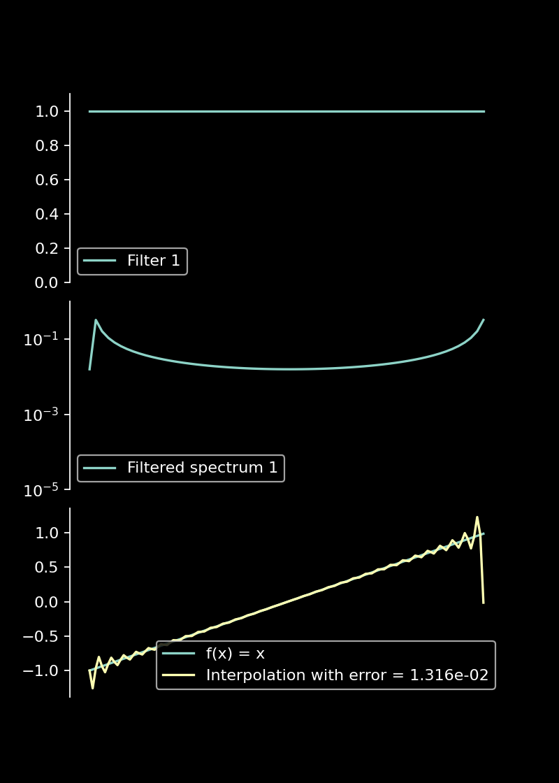
When the spectrum is filtered with a constant function, the decay of the Fourier coefficients is not modified. Accordingly, we can observe Gibb’s phenomenon.

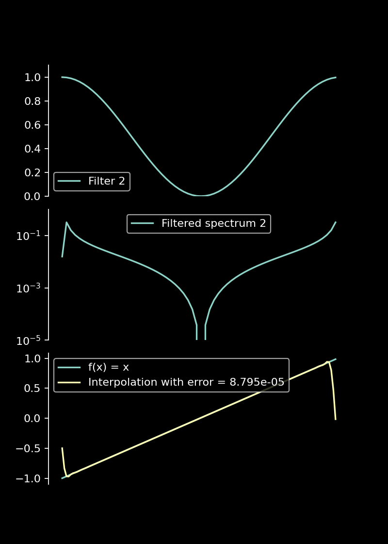
Filtering with a smoothly decaying filter function significantly reduces oscillations and increases the accuracy of the reconstruction.

Code

# import libraries
import numpy as np
import scipy
import scipy.integrate
from scipy.fft import fft, ifft
import matplotlib.pyplot as plt
plt.style.use('dark_background')

def sigma0(eta):
    return np.ones(eta.shape)

def sigma1(eta):
    return 0.5 * ( 1 + np.cos ( np.pi * eta ) )

filters = [sigma0, sigma1]

# Number of sample points
N  = 64
Ni = 128
x  = np.linspace(-1, 1, N,  endpoint=False)
xi = np.linspace(-1, 1, Ni, endpoint=False)

# Sampled function values
def func(x):
    return x
f = func(x)

def interpolate(y, Ni, s):
    N             = len(y)
    yhat          = fft(y, norm="forward")
    yhat_filtered = yhat * s
    Npad          = int(Ni/2 - N/2)
    yt            = np.fft.fftshift(yhat_filtered)
    ypad          = np.concatenate([np.zeros(Npad), yt, np.zeros(Npad)])
    ypad          = np.fft.fftshift(ypad)
    yi            = ifft(ypad, norm="forward")
    return yhat, yi

# Plot the results
for i, filter in enumerate(filters):
    # Create sigma function for the current filter
    def sigma(x):
        k = np.fft.fftfreq(len(x))
        k /= np.max(np.abs(k))
        return filter(np.abs(k))

    fig, ax = plt.subplots(3, 1, figsize=(5, 7), dpi=160)
    s          = sigma(x)
    fhat, fint = interpolate(f, Ni, s)
    k = np.fft.fftfreq(len(x))

    ax[0].plot(s, label=f"Filter {i + 1}")  # Plot the filter
    ax[0].set_ylim(0, 1.1)
    ax[0].legend()
    ax[1].set_yscale("log")
    ax[1].set_ylim(1e-5, 1)
    ax[1].plot(np.abs(fhat) * s, label=f"Filtered spectrum {i + 1}")  # Plot the magnitude of the Fourier coefficients
    ax[1].legend()
    ax[2].plot(xi, func(xi), label="f(x) = x")  # Plot the error
    ax[2].plot(xi, fint, label=f"Interpolation with error = {np.mean(np.abs(fint[8:-8] - func(xi)[8:-8])):3.3e}")  # Plot the error
    ax[2].legend()

    for j in range(3):
        ax[j].spines['top'].set_visible(False)
        ax[j].spines['right'].set_visible(False)
        ax[j].spines['bottom'].set_visible(False)
        ax[j].get_xaxis().set_ticks([])

    fig.subplots_adjust(hspace=0.1)
    plt.savefig(f"figures/filter_{i+1}.png")
    plt.show()