Computers learning Tic-Tac-Toe using tables
In today's post, we study ways to play Tic-Tac-Toe using the minimax and Q-learning algorithms. We heavily draw on Carsten Friedrich's excellent notebook series to explore ways to make a computer play games such as Tic-Tac-Toe. I will gloss over some details, so please refer to Carsten's post for some more explanations. You may find the accompanying Python code on GitHub.
Minimax algorithm
First, we turn towards a benchmarking algorithm: the minimax algorithm. A minimax agent assumes that its opponent will play optimally—making the best possible moves to win. Faced with such a formidable adversary, the minimax agent chooses moves that minimize its own loss — hence the name. If victory is out of reach, the agent aims to at least avoid defeat. We will pitch the minimax agent against a random agent making random, legal moves to see how it performs.
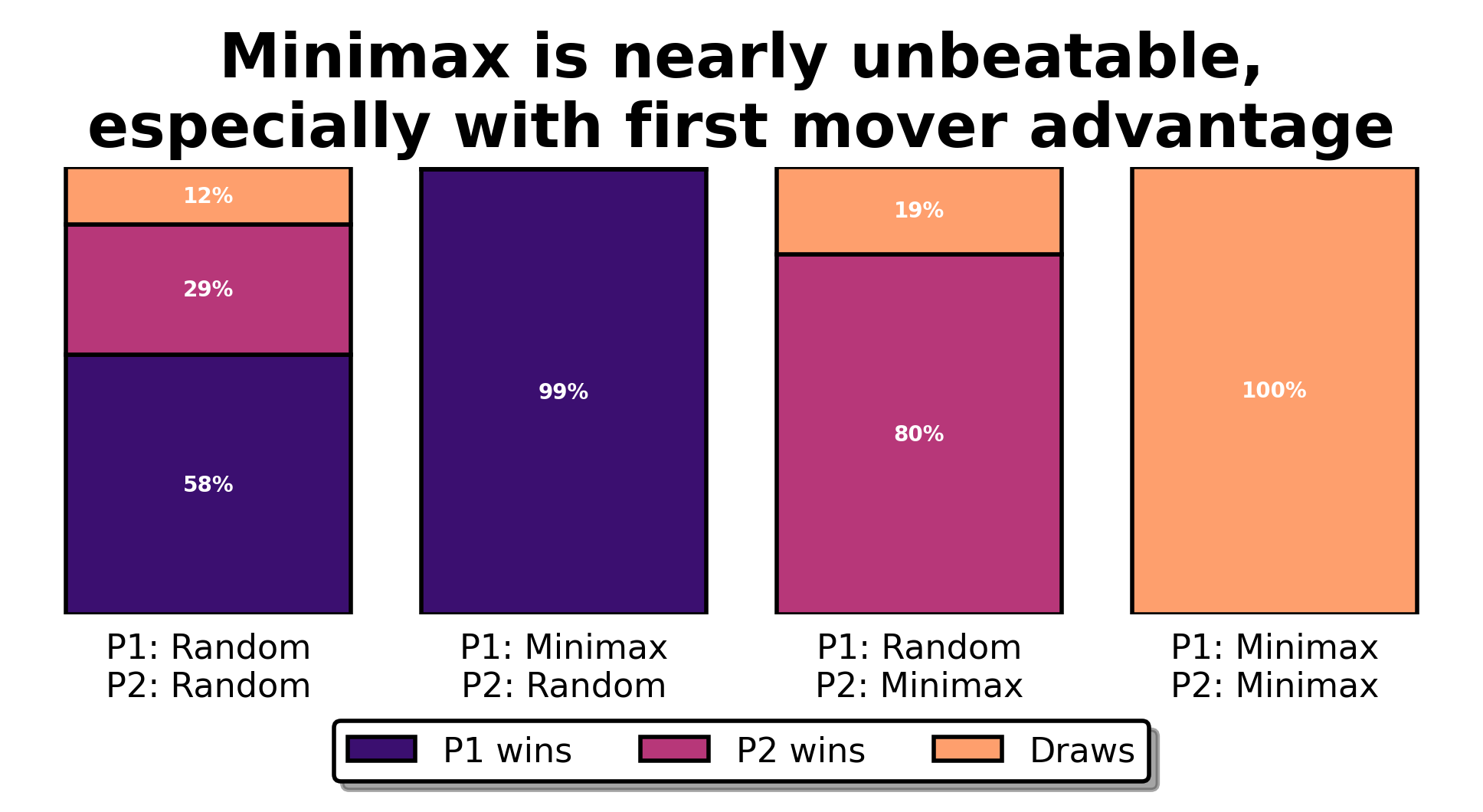
The above chart shows the results of 10000 games between the different agents. When two random agents play against one another, it turns out that the first player making a move has a significant advantage. The minimax agent playing first against the random agent is therefore nearly unbeatable. Going second, it stumbles into draws 20% of the time, but will never lose. Finally, the minimax agent achieves 100% draws when playing against itself. You can marvel at its performance in the introductory animation. But how does this black magic work?
How does the minimax agent decide which move to make?
The minimax algorithm works by evaluating all possible future game states. In a game like Tic-Tac-Toe, this means exploring up to \(3^9=19683\) board configurations—since each of the \(9\) squares can be in one of three states: X, O, or empty. The algorithm assigns a score to each final state (win, loss, or draw), and then works backwards from these terminal states to the current position, assuming both players choose optimally at every turn. Ultimately, it selects the move that leads to the best achievable outcome.
The name minimax comes from this interplay: the agent tries to minimize the possible maximum loss, while the opponent tries to maximize its own gain. It’s a game of antagonistic optimization. In Tic-Tac-Toe, this equals to assuming that the opponent will play perfectly and the best the agent can do is avoid defeat and aim for a draw. This sounds like a perfect strategy for all two-player, turn-based games, right? Well—yes, in theory. But the major drawback is computational cost. Even in a simple game like Tic-Tac-Toe, the number of potential board configurations (though reducible due to symmetries) is non-trivial. In complex games like chess, the explosion in possibilities is extreme. If we imagined each square having exactly \(6\) possible states (empty, rook, bishop, knight, queen, pawn), we get \(6^{64}\propto 10^{49}\) combinations.
To make minimax tractable in such cases, practical implementations use optimizations such as pruning (e.g., alpha-beta pruning) and heuristics to evaluate only a subset of promising positions. And what can stop a minmax agent? Well, another minmax agent as we have seen above. But it turns out that we can also do better against a random agent. We will see how in the next section.
Q-Learning
Now that we know what performance an agent needs to achieve to be better than a random agent and to play optimally, we can turn towards Q-Learning. While minimax works by exhaustively simulating all future outcomes, Q-learning takes a very different approach: instead of reasoning through every possible scenario, it learns from experience. More specifically, it learns how good a move is, so it can choose the best one at each step. But how do we measure that?
We define the Q-value as the total expected reward an agent will get by taking an action in a given state and then always acting optimally after that. Let’s say you’re in a certain board position and you decide to place your mark in the center. You might not win immediately, but this move might lead to a win 3 turns later. The Q-value reflects that.
So, given a table where:
- Columns represent the different board configurations (the states),
- Rows represent the different moves (the actions),
- Values are the Q-values that tell you how good an action is in a given state
you just pick the action with the highest Q-value in a given state and you are guaranteed to maximise your expected reward. Easy, right? Now, if you knew the Q-values from the start, things would really be easy. But unfortunately, you don’t.
Rather, you start with a random table or just set all Q-values to the same value and update them as the agent plays games and receives feedback. Over time, the agent learns to prefer actions that are more likely to lead to positive rewards, even without knowing all possible outcomes of the game. This makes Q-learning especially powerful in larger environments where minimax is computationally infeasible.
The Q-agent outperforms the minimax agent?
Before we dive into the details of Q-learning, let’s train a Q-learning agent by letting it play up to 10,000 games against a random agent and observe how it gradually improves.
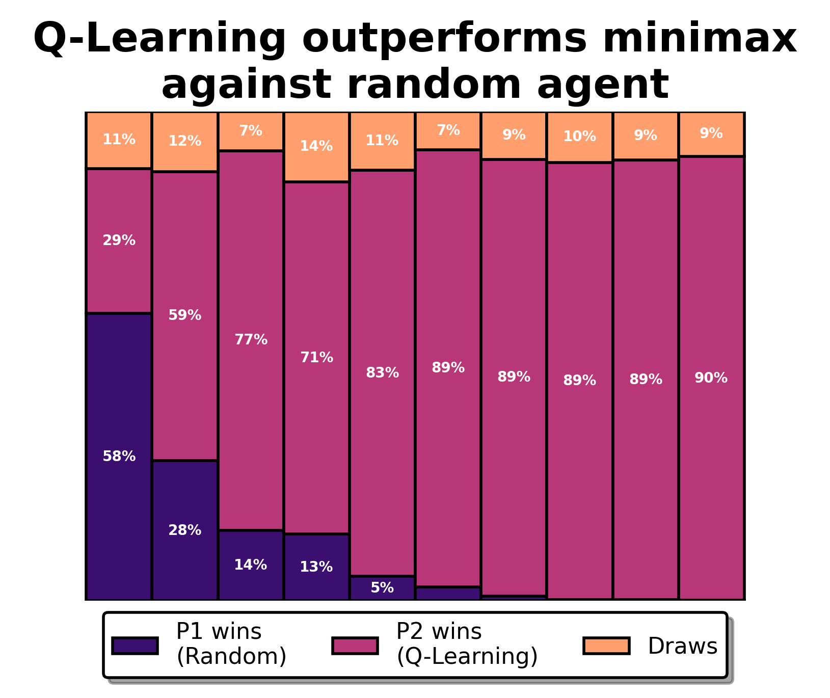
Surprisingly, it achieves close to 90% victories playing second against a random agent, whereas the minimax agent only achieved 80%. How is this possible?
Unlike minimax, which assumes the opponent plays perfectly, Q-learning can adapt to the behavior of different opponents—making it well-suited for environments where opponents are unpredictable or not fully rational. In this case, it observed that the random agent makes many mistakes and it takes full advantage of these by playing riskier than the minimax agent. That means it cannot avoid the occasional loss, but it performs better overall.
Interestingly, its risky strategies still hold up against the minimax agent, achieving 100% draws. Alternatively, we can also train the Q-agent directly with the minimax agent, and it still learns to play draws reliably.
How does the Q-agent learn about its environment?
The Q-value \(Q(s, a)\), given a state \(s\) where we take the action \(a\), is updated using the Bellman equation:
\[Q_{\text{new}}(s, a) = r + \gamma \cdot \max_{a'} Q(s', a'),\]where:
- \(s'\): next state after taking the action,
- \(r\): reward received after the transition,
- \(\gamma\): discount factor \((0 \leq \gamma \leq 1)\),
- \(\max_{a'} Q(s', a')\): the estimated value of the best action in state \(s'\).
This update nudges the old value of \(Q(s, a)\) toward a target value:
\[\text{Target} = r + \gamma \cdot \max_{a'} Q(s', a').\]Now, consider a case where the action \(a\) taken in state \(s\) leads directly to a win—meaning \(s'\) is a terminal state and the game ends immediately. In this case, the agent receives a reward of \(r = +1\). Since \(s'\) is terminal, there are no valid next actions, so:
\[\max_{a'} Q(s', a') = 0.\]Therefore, the Bellman update simplifies to:
\[Q_{\text{new}}(s, a) = 1 + \gamma \cdot 0 = 1.\]In other words, the Q-value for a winning move is updated toward 1, reflecting the fact that this action directly results in the most favorable outcome. The agent will learn to strongly prefer this action in similar states in the future. This is a form of bootstrapping: the agent improves its estimates using its current estimates of future outcomes.
Can we give a theoretical justification for this update? Yes, we can.
We begin by assigning scalar rewards:
- +1 for winning,
- 0 for drawing,
- –1 for losing.
A rational player would try to win as often as possible and avoid losing, thereby maximizing the cumulative reward across a game.
A naive way to define the cumulative reward from time step \(t\) is:
\[R_t = \sum_{k=0}^{\infty} r_{t+k}.\]However, in more complex games (e.g. a shooter), there may be intermediate rewards—like damaging an opponent—which should not be valued equally with final outcomes. To account for this, Q-learning introduces discounting with a factor \(\gamma\), defining the discounted return as:
\[G_t = r_t + \gamma r_{t+1} + \gamma^2 r_{t+2} + \cdots = \sum_{k=0}^{\infty} \gamma^k r_{t+k}.\]The discount factor balances the trade-off between immediate and future rewards:
- \(\gamma = 0\): only immediate rewards are considered.
- \(\gamma = 1\): future rewards are valued equally with current ones.
In Tic-Tac-Toe, where rewards occur only at the end, setting \(\gamma = 0\) means the agent receives no feedback for non-terminal moves. As a result, all intermediate actions seem equally ineffective. On the other hand, \(\gamma = 1\) allows the agent to learn that certain early moves can lead to a win several steps later—making them highly valuable.
If we accept the cumulative return \(G_t\) as a valid measure of long-term success, we can formally define the Q-value as:
\[Q^\pi(s, a) = \mathbb{E}_\pi \left[ G_t \mid s_t = s, a_t = a \right],\]where \(\pi\) is a policy—a rule for choosing actions (such as random play, greedy strategies, or minimax). The optimal Q-value is then:
\[Q^*(s, a) = \max_\pi Q^\pi(s, a).\]Now, observe that the return \(G_t\) is recursive:
\[G_t = r_t + \gamma G_{t+1}.\]Substituting this into the definition of \(Q^\pi(s, a)\) gives rise to the Bellman equation, which relates the value of a state-action pair to the expected reward plus the value of the next state. This recursive structure is what enables Q-learning to propagate final outcomes back to earlier decisions, allowing the agent to learn effective long-term strategies over time.
What parameters do we need to worry about?
Tabular Q-learning introduces a number of hyperparameters:
- Learning rate (α): Tabular Q-learning is not very sensistive to the learning rate and allows values closer to 1 (here: 0.01)
- Training frequency: I find that between 30,000 and 50,000 games with training every step work well.
- Discount: For Tic-Tac-Toe, there are only final and no intermediate rewards, so the discount is not independent from the rewards (here: 0.8).
- Initial Q-values: Higher initial Q-values foster more exploration, a value closer to zero leads to conservative and potentially slower training (here: 0.6)
- Exploration: During training, we do not always want the agent to strictly follow the Q-table. It can prove advantageous to let it randomly pick actions to further explore the state space (here: start with 100% exploration (random moves every move) that decreases by 1% every game and goes down to 0%-10% exploration)
What do Q-tables look like?
We can gain deeper insights into the Q-agent’s strategies by visualising the Q-table as a heat map.
What should you notice about the Q-agent’s Q-table?
- Invalid moves: Invalid moves are indicated by white cells (occupied positions).
- States with zero valid moves: I excluded all states with zero moves in this visualisation.
- Tic-Tac-Toe has \(3^9 = 19,683\) states of which only \(5,478\) are valid reachable states
- The visualisation shows half of these reachable states since it only shows the Q-table for an agent playing second
- Ordering: States are ordered by number of valid moves left.
- Initial Q-values: Many entries are orange: this corresponds to the initial Q-value of \(0.6\), chosen to balance exploration and conservatism.
- Rarely visited states: Early states with few or no visits such as the ones on the left retain their initial values.
- Strong positions: The agent strongly favors the center unless it’s already taken—then it prefers corners.
- Late game: As more opponent moves are added, the agent learns to avoid traps and block wins.
- Final game: Final states may include Q-values of \(-1\) (unavoidable loss), \(0\) (draw), or \(1\) (win).
We visualize the Q-values for a minimax agent for comparison. This can be done by visiting every state and asking the minimax algorithm what the ideal game outcome be for the player given its magnificent opponent.
How does the minimax agent’s Q-table differ from the Q-agent’s?
- High pessimism: The minimax agent assumes the opponent plays optimally. Accordingly, there are more zero or negative Q-values compared to the optimistic Q-agent trained on random play.
- Late game: Q-values reflect draws in most 8-move states.
Finally, training the Q-agent as second player against the minimax agent allows us to compare both tables more easily. For the sake of this experiment, we make the minimax agent deterministic: It always picks the same optimal action instead of randomly selecting one of the many optimal actions at its disposal in many states. This dramatically shrinks the number of states the Q-agent visits.
The Q-table obtained this way is directly comparable to the minimax agent’s Q-tables since the Q-agent was trained against an agent making optimal moves, i.e. it does not assume it can win games in case the opponent makes a mistake.
The minimax agent’s and Q-agent’s Q-tables match fairly well:
- Shared pessimism: Maximum Q-values are close to \(0\) in both cases and match
- Reliable draws: Q-agent reliably has learned to reliably play draws against the deterministic minimax agent
Conclusion
This post explored how the minimax and Q-learning algorithms can be used to teach computers how to play Tic-Tac-Toe. In the next post, we are going to look at Deep-Q-Learning approaches that replace the explicit Q-table by a regression algorithm using neural networks.