In this blog's first post, we are going to visualise a complex Fourier transform as sum of plane waves.

Intro

Discrete Fourier transforms are ubiquitous in image and signal processing. They allow the decomposition of a time-dependent signal into a sum of plane waves with constant frequencies. Today, we are going to visualise them in a cool neon-look using Python. I recommend the the excellent explanatory videos on the Fourier transform by the Youtube channel 3Blue1Brown where I first came across this type of visualisation. 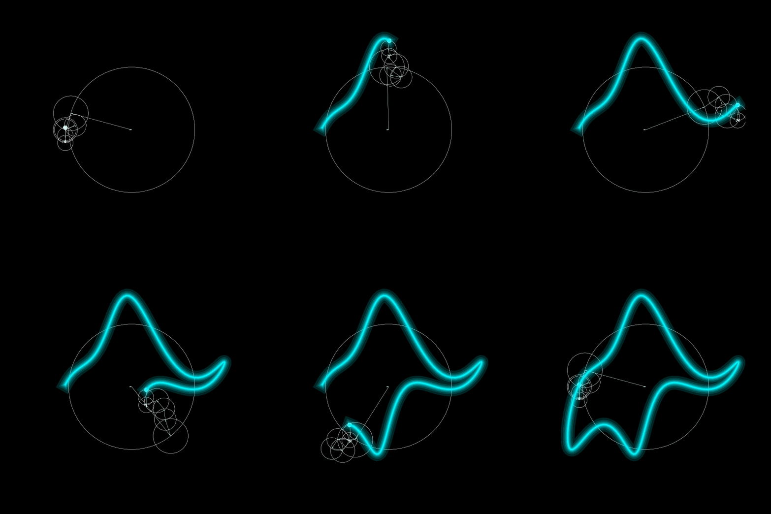Before diving in, below is a gif showing an animation of our result: You may find the accompanying Python code on GitHub .

Discrete Fourier transform

The one-dimensional discrete Fourier transform (DFT) and its inverse (IDFT) are defined as
\(\hat{f}(k) = \sum_{t=0}^{N-1} f(t) \cdot e^{-i 2 \pi t n/N}\)
\(f(t) = \frac{1}{N} \sum_{k=0}^{N-1} \hat{f}(k) \cdot e^{+i 2 \pi k t/N}\)
for a function \(f\) taking real or complex values, \(N > 0\) and \(0 \leq t, k < N\). How to interpret these equations? Each frequency \(k\) corresponds to a vector of constant length \(\frac{1}{N} \hat{f}(k)\). At a given time, it points in the direction of the plane wave \(e^{+i 2 \pi k t/N}\), that is, the point \((\cos(2 \pi k t/N), \sin(2 \pi k t/N))\) in the complex plane. The sum of plane waves is equal to adding the vectors with the sum of vectors pointing to the complex number \(f(t)\). Time evolution implies that each vector rotates at constant speed tracing a circle.

Drawing an Elephant

This equips us with the knowledge to get started: We take the discrete Fourier transform of a periodic (\(f(t) = f(t + \delta t)\)), time-dependent input function. Our input function \(f(t)\) is von Neumann’s 4-parameter elephant based on the paper “Drawing an elephant with four complex parameters” by Jürgen Mayer et al. (2010, DOI:10.1119/1.3254017).

import numpy as np 
import matplotlib.pyplot as plt

# set up input data
def elephant(t):
    y =  50*np.sin(t)+18*np.sin(2*t)-12*np.cos(3*t)+14*np.cos(5*t)
    x = -60*np.cos(t)+30*np.sin(t)  - 8*np.sin(2*t)+10*np.sin(3*t)
    return x/100 + 1j*y/100

# number of points at which to sample elephant
N      = 128
times  = np.linspace(0, 2 * np.pi, N+1)
# compute time-series data for elephant
f      = elephant(times)
# compute Fourier transform excluding f[-1] == f[0]
fHat   = np.fft.fft(f[:-1])

In the next step, we compute the IDFT at a given time by first calculating an array containing the plane waves with the magnitudes calculated by the DFT and then sort them from low to high frequencies.

# time at which to evaluate IDFT
t      = 64 
# plane waves with coefficient determined by FFT of input data 
waves  = fHat*np.exp(1j*2*np.pi*t*np.arange(N)/N)/N
# returns frequencies corresponding to entries of fHat
# for N even: 0, 1, 2, ..., N/2, -N/2 - 1, ..., -1
freqs  = np.fft.fftfreq(N)
# sort waves by magnitude of frequencies from slow to fast 
waves  = waves[np.argsort(np.abs(freqs))]

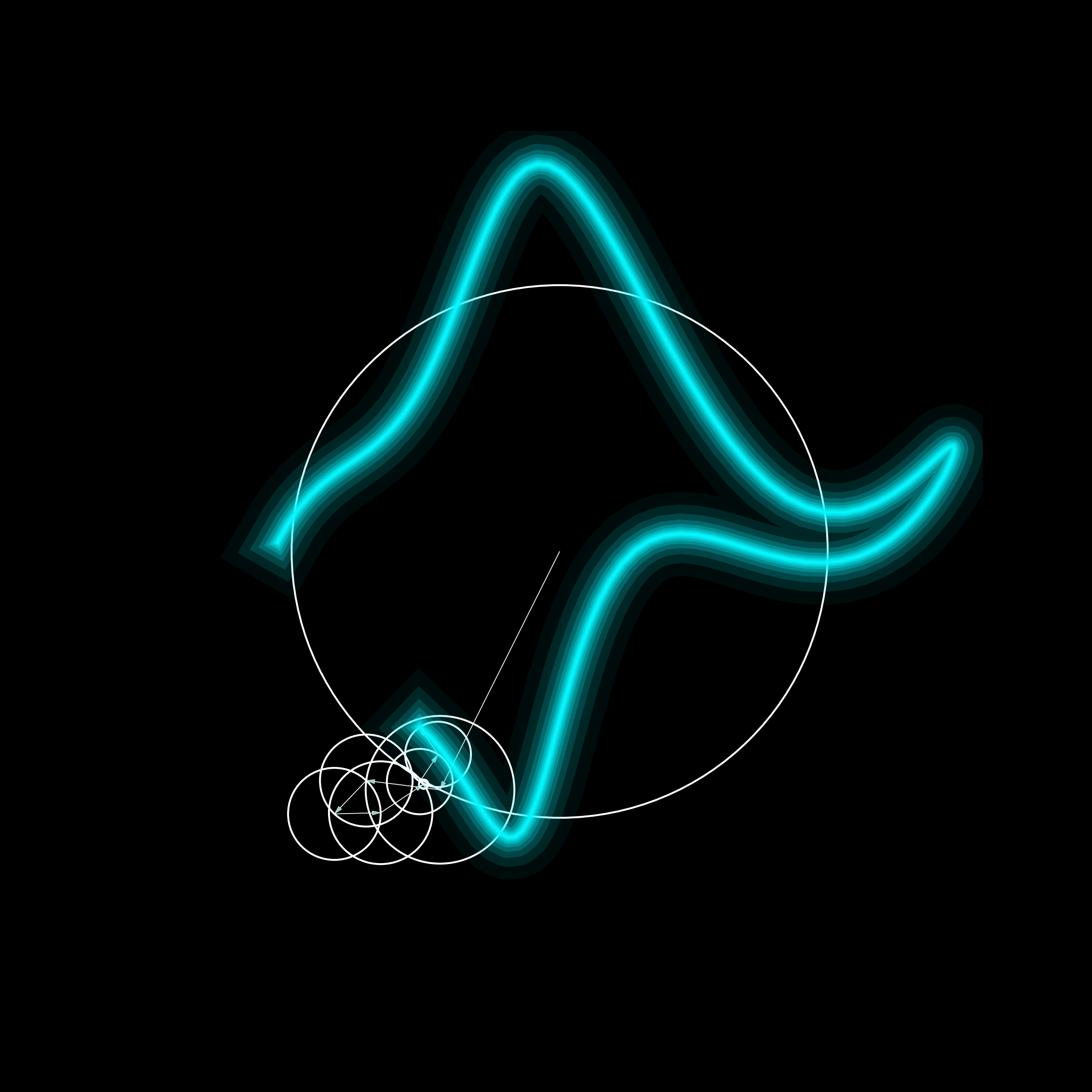
Finally, we plot the elephant as well as the vectors the plane waves describe and the circles they trace:

# create figure
fig, ax = plt.subplots(dpi=600)
plt.axis("off") 
plt.style.use('dark_background')

# plot elephant in neon-look 
# credit to Dominic Heitz at TowardsDataScience
linewidths     = np.logspace(-5, 5, 20, base=2)
transparencies = np.linspace(+1, 0, 20)
for lw, alpha in zip(linewidths, transparencies):
    plt.plot(np.real(f[:t+1]), np.imag(f[:t+1]), \
             lw=lw, alpha=alpha, c='#08F7FE')
    
# first vector starts at origin
x      = 0
y      = 0
# do not show vectors shorter than cutoff
cutoff = 1e-2

# sum over plane waves
for i in range(N):
    # determine direction of vectors 
    dx = np.real(waves[i])
    dy = np.imag(waves[i])

    # do not show very short vectors
    if np.abs(waves[i]) > cutoff:
        plt.arrow(x = x, y = y, dx = dx, dy = dy, lw = 0.1,\
                  head_width=0.01, head_length=0.02,\
                  length_includes_head=True)
        ax.add_patch(plt.Circle((x,y), np.abs(waves[i]), \
                     fill = False, lw=0.5))

    # sum up plane waves
    x += dx
    y += dy

plt.savefig("elephant.png")

The final result looks as follows: If you like you can play around with the code and use different input data. Have fun!