In today's post, we study ways to play Tic-Tac-Toe using different deep Q-learning algorithms using dual networks, duelling networks, convolutional networks and prioritised experience replay. Just as in the previous post, we heavily draw on Carsten Friedrich's excellent notebook series to explore some reinforcement learning algorithms in more depth. I will gloss over some details, so please refer to Carsten's post for some more explanations. You may find the accompanying Python code on GitHub.

Deep Q-Network

The idea of Deep Q-Network (DQN) is simple: Instead of having a table that directly stores the Q-values as in the case of tabular Q-learning, we use a regression algorithm to approximate the table. The underlying algorithm stays the same, but instead of directly updating the values in the table, we give the regression algorithm information about how the Q-values should be updated. The advantage? While it is possible to have a table for all actions and states for a simple game like Tic-Tac-Toe, in a more complex setting the state space grows far too quickly and we need some low-dimensional approximation. In principle, any regression algorithm can be used for the task, but this algorithm uses neural networks. Hence the name Deep Q-Network. There are a number of reasons why one would choose neural networks over decision trees or a nearest-neighbour algorithm etc.:

• Scalability to high-dimensional inputs: Neural networks can handle large, continuous, or high-dimensional state spaces, especially when states are images or sensor arrays.
• Generalization: NNs can generalize from seen to unseen states, rather than memorizing exact values. This is crucial in environments where each state is encountered at most once.
• End-to-end learning: They can learn directly from raw input without the need for manual feature engineering, making them ideal for tasks like vision-based control.

Compared to tabular Q-learning, DQN-learning can become unstable or even diverge and it may misestimate Q-values, especially in underexplored regions. So, whenever you have the option to use tabular Q-learning, go for it. It is more stable and often provides better results – even if you have to manually craft features to describe the state-space in my experience.

You’re not just learning from experience — you’re trusting an approximator that you don’t understand to make up values you haven’t seen.

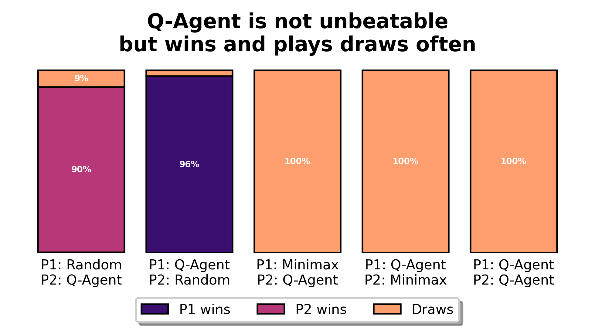
Given that we are approximating a Q-table, we can benchmark all deep Q-learning algorithms against the tabular Q-agent whose performance is summarised by Figure 1 below.

What changes compared to tabular Q-learning?

In tabular Q-learning, the Q-values are updated using the Bellman equation:

In DQN, we replace the Q-table with a neural network \(Q_\theta(s, a)\) parameterized by weights \(\theta\), and minimize the mean squared error loss between the predicted Q-value and the target:

where the target value is:

Here, \(Q_{\theta^-}\) is the target network (a periodically updated copy of the Q-network) used to stabilize learning.

Compared to tabular Q-learning, DQN introduces additional design decisions and hyperparameters:

• Learning rate (α): Typically lower than in tabular Q-learning (here: 0.01) to avoid destabilizing the NN updates.
• Neural network architecture: For this benchmark, we use TensorFlow Keras for a fully-connected network with a single hidden layer of 64 neurons and ReLU activation with Adam optimiser and mean-squared error.
• Replay buffer: Stores past transitions (here: up to 10,000) and allows sampling mini-batches (here: 128 once there are at least 1,000 transitions) to break temporal correlations.
• Gradient updates: Number of gradient updates per training step (here: usually 3,000 games with training every game and two gradient updates per training)

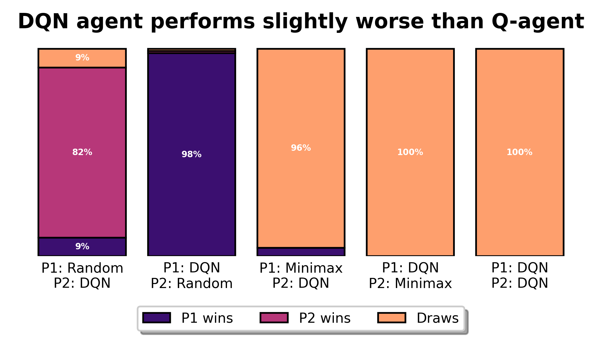
I will touch upon the topic of hyperparameters in a follow-up post, but rest reassured that they require fine-tuning. If everything goes well, you will find results as shown in Figure 2. Note that in this simple example, the training of the DQN agent is more computationally expensive than training the tabular Q-agent.

What does the DQN agent’s Q-table look like?

As in the case of tabular Q-learning, we can sample the neural network at every state to obtain the Q-values for all actions and visualise them. Ideally, the table should approximate the Q-table shown in Figure 3 in the previous post.

We observe the following differences:

• Value range: The heatmap spans values from roughly \(-7\) to \(4\) — far beyond the actual game reward bounds of \([-1, 1]\). This is expected: a neural network approximates Q-values via regression and isn’t constrained to output within the range of real returns. Still, we’d expect a well-tuned model to eventually converge toward the true Q-table and not exhibit such large deviations.
• Generalisation: I didn’t grey out invalid or unreachable states to highlight that the network infers Q-values for all possible states — whether visited or not. It also assigns values to invalid actions, despite those being masked during training and inference. This reflects the generalisation behaviour of neural nets: they don’t just remember, they predict.

As before, we also train the DQN agent as second player against the deterministic minimax agents and show the reduced Q-tables.

A few remarks about the DQN agent’s Q-table shown in Figure 4:

• Bias from the opponent: In Figure 4, the DQN develops a strong bias against the top-left move — that’s because the minimax opponent always plays there first. Since this move is illegal for the DQN during training, it never gets updated and remains a leftover artefact of random initialisation.
• Drawing states: In the few drawing states — \(0\), \(7\), \(10\) and \(25\) — the DQN mimics the minimax agent reliably and achieves draws. So even if value estimates are noisy, the learned policy is solid.
• Noisier values: Overall, the Q-values are noisier than those of the tabular agent — an inevitable consequence of using regression instead of direct updates.

To conclude this post, we visualise the table shown in Figure 4 during the training process:

Conclusion

This post explored how the DQN algorithm can be used to teach computers how to play Tic-Tac-Toe. In the next post, we are going to explore the choice of hyperparameters, the training process and more advanced versions of the DQN algorithm in more detail.