Computers learning Tic-Tac-Toe Pt. 3: Optimisation
In the previous post we built a simple Deep Q-Network (DQN) agent for Tic-Tac-Toe and compared it to its tabular cousin. Today, we look at its hyperparameter optimisation as I find that as all the seemingly arbitrary hyperparameter choices in machine learning algorithms are a fascinating but also unsettling topic. We first study a flame graph of a DQN training run and then use the Optuna hyperparameter optimisation framework with the single-network DQN model.
Performance optimisation
In the following, we study whether the performance of our simple single-network DQN algorithm can be improved. Before we start, it is important that highlight that you should not waste your time or sacrifice the readability of your code for optimisations that turn out to be worthless. In the words of Donald Knuth:
We should forget about small efficiencies, say about 97% of the time: premature optimization is the root of all evil. Yet we should not pass up our opportunities in that critical 3%.
Flame graphs are a visualisation of the stack trace of a profiled software created by Brendan Gregg. They allow you to identify performance bottlenecks in your code visually with minimal effort. And flame graphs help to identify the 3% of opportunities Knuth talked about! Let us take a look at a flame graph of my DQN learning routine created with the wonderful py-spy. It is great for interactive vector graphics. For a conventient local analysis, I also recommend snakeviz.
In this run, the run_training function dominates the execution time. Most of it is consumed by the train function of the vanilla DQN, which itself relies heavily on TensorFlow’s predict_on_batch and train_on_batch. Since these are well-optimized internals, any inefficiency likely stems from misuse (e.g. improper input formatting or inefficient batch sizes).
Another chunk of time is spent in the minibatch_to_arrays function, which converts Python lists to TensorFlow arrays. While this might be optimisable, it only accounts for ~30% of execution time — not worth pursuing unless necessary.
Similarly, the act function takes time due to TensorFlow inference calls, which again is expected. One worthwhile optimisation I did make: disabling TensorBoard, which drastically cut training time from 10 to 2 minutes.
Hyperparameter optimisation
Hyperparameter tuning is the less glamorous sibling of model design, often feeling like adjusting dials in the dark hoping for gold. With parameters like learning rate, discount factor, batch size, and exploration decay all in play, brute-force grid search quickly becomes infeasible.
Still, grid search can be illuminating — especially for sensitivity analysis around a known good configuration. The plot below shows the result of sweeping various hyperparameters individually, with all other parameters held constant from the previous post.
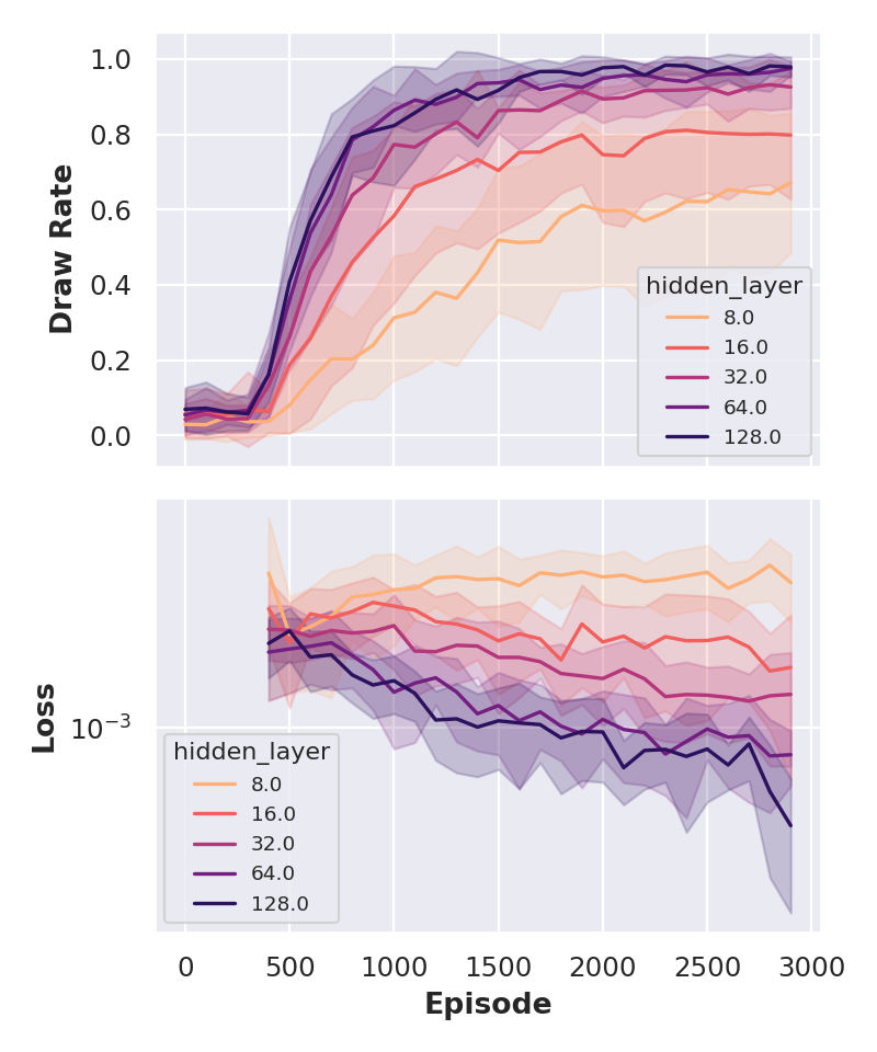
We observe several things:
- Hidden Layer Size: At least 64 neurons are needed for good performance. Larger networks reduce training loss due to more degrees of freedom but risk overfitting. In the following, I will use a single layer with 128 neurons.
- Learning Rate: Even with Adam optimiser, this hyperparameter is critical. Too high, and training diverges. Too low, and it crawls. The best-performing configuration also yields the lowest loss. In the following, I will use a learning rate of 0.003 as default.
- Gradient Steps: The number of updates per training step has a limited effect. Fewer updates slow convergence slightly, but the final performance remains largely unchanged. In the following, I will use two gradient steps.
- Discount Factor: Affects convergence speed but not end performance — at least in this setup. It is correlated with the learning rate, likely due to their joint influence on value estimation. In the following, I will use a discount factor of 0.8.
- Exploration Decay: Too low a decay hampers training, as the agent stays random for too long. Otherwise, it has little effect — slower decay could simply require more training. In the following, I will use an exploration decay of 0.01 to a minimum exploration of 0.1.
- Batch Size: Has minimal influence on performance but impacts training loss. Larger batches reduce variance in gradient updates and thus loss, but may lead to overfitting in more complex environments.
These results raise an important question: What about interactions between hyperparameters? Could a smaller network outperform a larger one with the right discount and learning rate, for instance?
To answer this, I turned to the elegant Optuna framework. Optuna uses intelligent sampling of the search space and supports early pruning of poor runs — making it a great fit for expensive training pipelines. We can set up a study a by specifying and optimisation goal and the hyperparameters to change. After some experimentation, I chose the average draw and victory rate across five training runs for every trial: DQN vs random, random vs DQN, DQN vs Minimax, Minimax vs DQN and DQN vs DQN for every trial. We saw earlier that the training results also vary quite a bit depending on the random number generators, so averaging across several training runs is sensible to avoid falsely identifying an outlier as good parameter set. Still, also averaging over different random number generator seeds would be even better, but time-consuming. The results of the optimisation that ran for 12 hours looks like this.
Following our earlier results, I focused on three parameters I deemed interesting: the learning rate, the discount and the number of neurons in the hidden layer where we keep one hidden layer. The following plots show the breakdown of the optimisation results by these three variables.
The plot suggests some trends that we can verify with a linear regression: \(\text{objective} = \beta_0 + \beta_1 \cdot \text{learning rate} + \beta_2 \cdot \text{discount} + \beta_3 \cdot \text{hidden units} + \varepsilon,\) where \(\text{objective}\) is the average draw rate across evaluation games, \(\beta_0\) is the intercept (baseline performance) and \(\varepsilon\) is the unexplained error (residuals).
The table below summarizes the model coefficients and global fit statistics:
| Term/Metric | Value | p-value | Interpretation |
|---|---|---|---|
| Intercept | 0.56 ± 0.08 | < 0.1% | Baseline performance when all params are 0. |
| Learning Rate | 9.8 ± 3.5 | 0.7% | Increasing the learning rate leads to a strong improvement of the result — as long as it’s not too high and unstable |
| Discount Factor | 0.18 ± 0.01 | 7.5% | Moderate effect. Not statistically significant at 5% level, but borderline. |
| Hidden Units | 0.043 ± 0.011 | < 0.1% | More hidden units improve the results. |
| R-squared | 0.275 | — | 27.5% of the variation in draw rate explained by the model. |
| Adjusted R-squared | 0.245 | — | Adjusts for the number of predictors. |
| F-statistic | 9.348 | < 0.1% | Tests if at least one predictor has a non-zero effect. p-value is low - the model is statistically significant |
Finally, we can also try to understand more non-linear effects with a parallel coordinate plot, for instance. You can select parameter ranges like the one for 32 hidden units, for instance, and it becomes obvious that 32 hidden neurons give bad results regardless of the learning rate and discount.
Conclusion
In this post, we explored techniques for optimizing both the performance and hyperparameters of a single-network DQN agent. For performance tuning, I strongly recommend using flame graphs — they’re an excellent way to spot bottlenecks and inefficiencies in your implementation.
When it comes to hyperparameter optimization, nothing beats a good initial guess. Simple parameter sweeps are an effective way to check whether you’re operating near a “sweet spot.” While frameworks like Optuna are powerful and can help develop intuition about parameter sensitivity and interactions, they can also be computationally expensive.
In any case, it is imperative to limit the number of tunable parameters to fewer than 10 — ideally less than four or five — to avoid the curse of dimensionality.
To speed up experimentation, I recommend building a simplified toy model of your problem. You could, for instance, use a smaller, synthetic training set with a fixed number of transitions to control training time and constrain the state space and reduce network size to further accelerate benchmarking. These simplifications can dramatically reduce training time and help you iterate more quickly on model design and parameter tuning.
In the next post, we’ll move beyond tuning and look at how to improve the DQN algorithm itself.