Computers learning Tic-Tac-Toe Pt. 4: Towards Rainbow DQN
In the previous post we optimised our single-network Deep Q-Network (DQN) agent. Today we level-up that agent with three classic extensions that address DQN’s biggest pain points: Double DQN, Dueling DQN and Prioritised Experience Replay.
Before diving into improvements, we also add vanilla DQN — i.e. the correct implementation with two separate networks — as a baseline reference. Our earlier agent used a simplified setup where the target and online networks were identical (\(Q_\theta = Q_{\theta^-}\)), which is known to lead to instability. We now evaluate how much benefit we get by simply introducing the second network as originally proposed in DQN.
We study four setups in more detail:
- Vanilla DQN – two separate networks; a stable target using \(Q_{\theta^-}\)
- Double DQN – fixes systematic over-estimation of action values.
- Dueling DQN – separates what a state is worth from which action is best.
- Prioritised Experience Replay (PER) – replays the transitions that matter most.
Each idea is independent and inexpensive to bolt on, yet in combination they underpin most modern DQN-style agents (e.g. Rainbow).
Vanilla DQN – two networks for stability
Our original DQN agent used a single neural network for both action selection and temporal difference target (TD-target) calculation — i.e., we set the target and online networks to be the same (\(Q_\theta = Q_{\theta^-}\)). This made the implementation simple but deviated from the original design proposed by Mnih et al. (2015).
Vanilla DQN corrects this by maintaining two separate networks:
- The online network \(Q_\theta(s, a)\) is updated at every training step via gradient descent.
- The target network \(Q_{\theta^-}(s, a)\) is updated less frequently. Two common strategies are a hard update where the target network’s weights are are copied directly from the online network every N steps or a soft update or Polyak averaging where the weights of the target network are blended with the online network’s weights using a small constant \(\tau\) as \(\theta^- \leftarrow (1 - \tau) \cdot \theta + \tau \cdot \theta^-\).
This stabilises learning by preventing the TD-target from shifting too rapidly. Concretely, the target used in the loss is:
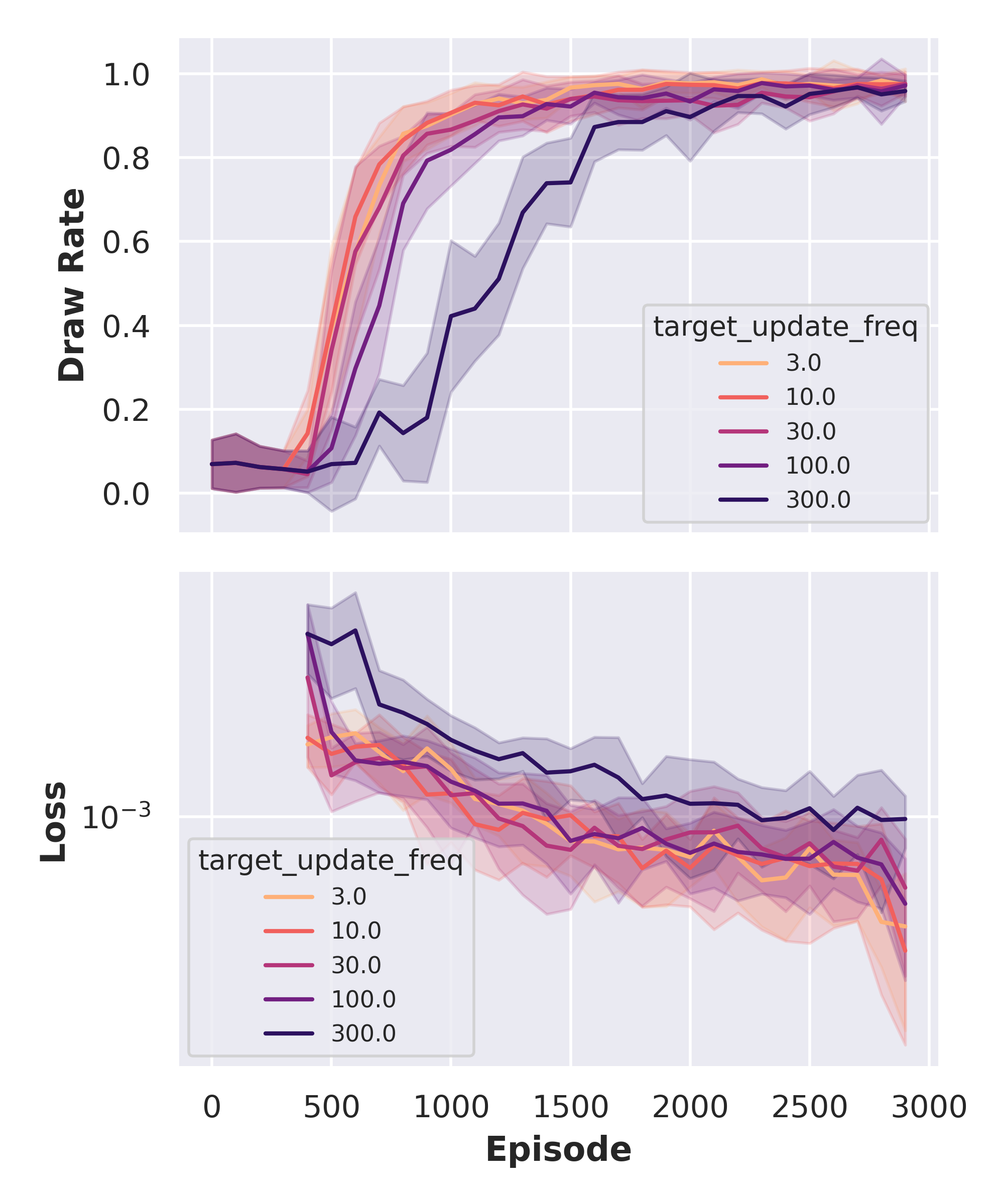
\[y_t = r_{t+1} + \gamma \max_{a'} Q_{\theta^-}(s_{t+1}, a')\]Only this change is required in code — but it makes a significant difference in convergence stability for environments with noisy rewards or longer horizons. In our Tic-Tac-Toe setting, the benefit is smaller, but we include it as a baseline for the later extensions. You can find a comparison of the influence of these update strategies below. In general, I do not find that the double network architecture improves the performance of our Tic-Tac-Toe agent but this is probably to be expected given that rewards are not sparse.
Double (Dual) DQN – tame the over-estimation bias
Vanilla DQN uses the same network to both select and evaluate the action inside the TD‑target
\(y_t \;=\; r_{t+1} + \gamma \,\max_{a'} Q_{\theta^-}(s_{t+1}, a').\)
Because the max and the value share parameters, positive noise is amplified, leading to overly optimistic Q‑values.
Fortunately, van Hasselt et al. (2015) propose a simple solution: We can decouple selection from evaluation by keeping two separate neural networks: an online network \(Q_\theta\) and a target network \(Q_{\theta^-}\). Empirically, the bias disappears and learning becomes more stable – especially in sparse‑reward games.
The online network chooses actions and the target network is used to evaluate how good they were.
\(a^* = \arg\max_{a'} Q_{\theta}(s_{t+1}, a') \quad\text{(online network chooses)}\) \(y_t = r_{t+1} + \gamma \, Q_{\theta^-}(s_{t+1}, a^*) \quad\text{(target network evaluates).}\)
Only this one‑line change is required in the learning update. While the performance of the network remains similar for Tic-Tac-Toe, I do detect a difference in the Q-tables shown in the figure below. As expected, the values in the Q-table reconstructed from the target network trained with Double DQN tend to be slightly lower than those of the target network reconstructed from Vanilla DQN
Duelling DQN – separate value from advantage
The introduction of duelling networks by Wang et al. (2016) was guided by the realisation that on many steps the choice of action barely matters (think: standing still in Pong between bounces). Yet, the vanilla Q‑network must still back‑propagate a distinct value for every one of those near‑equivalent actions. Wang et al. proposed a network that first produces a state‑value \(V_\phi(s)\) and an advantage vector \(A_\psi(s,a)\); it then recombines them into Q‑values:
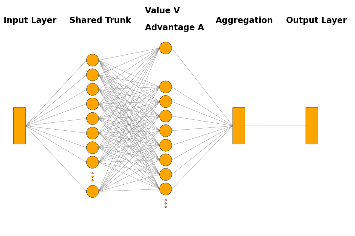
\[Q(s,a) \;=\; V_\phi(s) \;+\; \Bigl(A_\psi(s,a) - \tfrac{1}{|\mathcal A|}\sum_{a'} A_\psi(s,a')\Bigr).\]This “dueling head” lets the agent learn how good a state is even before it knows which action is best, speeding up credit assignment and generalisation. The network itself schematically looks as shown below: The input board state usually flows through one or several layers before being split up into the state-value and the advantage vector, possibly followed by more layers in both streams, before being aggregated according to the above equation and then sent to the output layer.
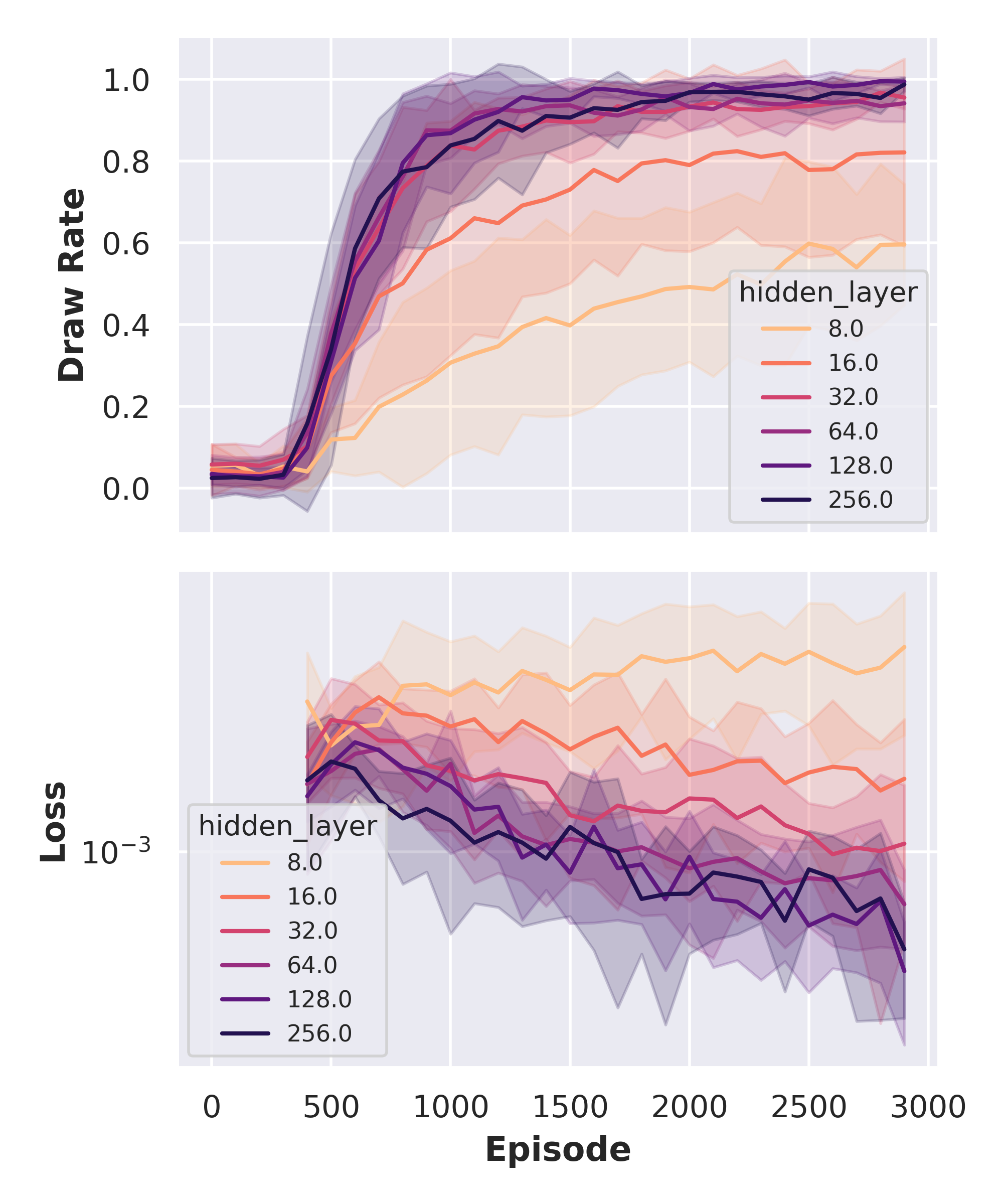
In my DQN implementation, I choose to represent both the value and advantage streams using two hidden layers with 128 neurons, each. I wondered whether the more complex network architecture would change the ideal number of neurons in these layers, but the parameter sweeü shown below suggests that fewer neurons mean worse performance.
What is interesting about the duelling netowrk architecture that we are training two separate outputs that we can query separately to study what they encode. Figure 5 shows both the learned state and advantage values.
Looking at the state values we see the following:
- The agent predicts the highest V-value for state 25 where it achieves a draw regardless of the next move. The V-value is close to 0 and the A-vector is close to 0 as well. Therefore, the remaining actions lead to Q-values close to 0 following Q = V + (A - mean(A)).
- State 0 has a high V-value of around -0.5. Playing center is the move with the highest A-value of around 0.5. The mean advantage, again, is close to zero as for all states shown here. Therefore, the Q-value of the center move is close to 0 - suggesting it can lead to a draw.
- There are a number of moves with high and low A-values in state 10 that has the third-highest V-value of around -0.5. Actions that lead to immediate defeat - bottom right, bottom center and center right have low A-values of around -0.5. The only legal move that avoids defeat - center left - has the highest action value translating into a Q-value of around 0.
These considerations show that the Duelling DQN agent has learned a sensible representation that separates how good a state is from which action is best. On Tic-Tac-Toe it achieves performance similar to the other DQN approaches I have introduced before. Please refer to the notebook for more plots.
Prioritised Experience Replay – learn more from what surprises you
In standard (uniform) replay, every past transition is equally likely to be sampled for training. But not all transitions are equally “useful”: A transition where your network’s Q-estimate is very wrong, i.e. it shows large temporal-difference errors (TD errors), carries more learning signal than one it already predicts well. Schaul et al. (2016) introduced Prioritised Experience Replay (PER) to replay such transitions more often, so your agent spends more gradient updates where it can learn most.
Imagine you are revising with flash‑cards. You naturally spend more time on the cards that keep tripping you up and only occasionally glance at the ones you already know. PER teaches a reinforcement‑learning agent to do exactly that.
In terms of implementation, we mainly need two elements - a priority for every transition and a way to sample transitions according to their priority. The priority is defined as
\[p_i = |\delta_i| + \varepsilon\]where \(\delta_i\) is the TD error and \(\varepsilon\) a small constant that ensures that transitions are visited once in a while even if their TD error is zero, i.e. even easy cards stay in circulation. The probabilities are then calculated as
\[P(i) \;=\; \frac{p_i^\alpha}{\sum_k p_k^\alpha},\]where \(\alpha\) controls how strongly to prioritise high TD error transitions (\(\alpha = 0\) → uniform). The need to sample with weights changes the requirements for our replay buffer. The simplest modification would be to implement a linear search: We store tuples of transitions and their priorities in a flat array. To pick items with a higher priority more often, we can add up all the priorities to get a total and pick a random number between 0 and that total. We then walk through the list, adding up priorities until the running total exceeds the random numbers. That is your selected item. Numbers with a higher priority are more likely to be picked and this likelihood scales linearly with the priority. Technically speaking, we define a probability distribution over items by normalising their priorities and compute the cumulative distribution function (CDF) which is just the running total of probabilities. This technique is called inverse transform sampling and can be used for generating sample numbers at random from any probability distribution given its cumulative distribution function.
In this approach, sampling has \(\mathcal{O}(N)\) time complexity in the buffer size \(N\) because we need to iterate over all elements. On the up-side, updating probabilites of a given transition works in constant time since we can directly index the relevant priority. Still, we are impatient and do not like linear time for sampling.
To cut sampling to logarithmic time we store the priorities in a complete binary tree where each parent holds the sum of its two children—the sum‑tree. The root therefore stores the sum of all priorities and picking a sample becomes a quick left‑right walk down the tree: To find a transition with a given probability, we pick a random number between 0 and the root node’s value.
- We pick the root node’s left child if the child’s value is larger than the random number.
- Else, we pick the right node and subtract the left node’s value from the random number.
- We continue this process until we reach a leaf node. That is your selected item.
Since we only explore one branch of the tree, the computational complexity is reduced from linear to logarithmic. The price to pay is that updating priorities now also comes at a logarithmic cost because we need to update all parent sums from leaf to root.
PER purposely breaks the i.i.d. assumption, i.e. that data points are independent and identically distributed. The i.i.d. assumption underlies most theoretical guarantees in machine learning and ensures that the training data is representative of the test data. If the agent mostly sees transitions with high TD errors, it might focus excessively on rare or exceptional situations and perform less well on more typical ones. In practice this bias is removed with importance‑sampling (IS) weights
\[w_i \;=\; \left( \frac{1}{N \, P(i)} \right)^{\beta},\]where \(N\) is the buffer size and \(\beta\in[0,1]\) controls the strength of the correction. The weight rescales the TD‑error of transition i before the gradient step. When \(\beta=1\) the update is unbiased; when \(\beta=0\) no correction is applied.
Because the largest weight can explode early in training, the common practise is to divide all weights by \(\max_i w_i\) so that \(w_i\in(0,1]\). Most implementations anneal \(\beta\) linearly from a small value (e.g. 0.4) to 1 over the course of training.
Early on the agent is like a student cramming the most difficult flashcards; later it wants a balanced rehearsal before the final exam.
Spoilt for choice: More hyperparameters
The three important PER hyperparameters are
| symbol | role | typical range |
|---|---|---|
| \(\alpha\) | strength of prioritisation | 0.4 – 0.7 |
| \(\beta_0\) | initial IS correction | 0.3 – 0.5 |
| \(\beta_{\text{steps}}\) | updates until \(\beta=1\) | few × 103 – 105 |
The interactive sweep below shows how they matter in the Tic‑Tac‑Toe experiment:
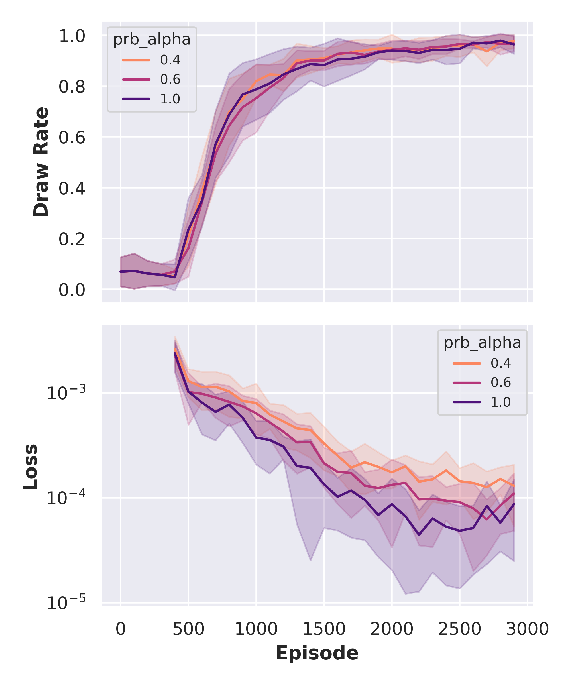
As you can see, the differences between different hyperparameters are marginal. This is because on Tic‑Tac‑Toe both vanilla DQN and PER‑DQN quickly discover a near‑draw policy, leaving few hard situations to learn from. To make the difference between the algorithms visible I therefore freeze a dataset of 10 000 random‑play transitions and train both agents offline. The tables in Figure 8 show how often each board state is replayed.
The figure suggests that PER visits the trivial opening position less often and spends more time on deeper boards. The corresponding TD‑error histograms in Figure 4 confirm the intuition: by replaying high‑error transitions more often PER flattens the right tail of the error distribution and equalises the visitation count across bins.
Since PER visits states with high TD errors more often, there are fewer states with high TD errors - the distribution is less extended to the right. Also, the number of state visits per TD error quantile is distributed much more evenly for the PER algorithm.
Putting it all together
Double DQN, Dueling networks and Prioritized replay complement each other neatly. In fewer than fifty lines of code you can
- compute the TD‑target with Double DQN,
- swap the value‑function head for a Dueling head, and
- replace the FIFO buffer with the PER sum‑tree.
On large, noisy tasks this trio is usually both faster to learn and better at convergence than plain DQN. On tiny tabular games such as Tic‑Tac‑Toe the gains are minimal—a tabular Q-agent still wins.
In the next post we will take the upgraded agent to a tougher arena: Bomberman. From there the road leads toward the full Rainbow combination with multi‑step returns, noisy nets and distributional value functions.