Computers learning PDEs Pt. 1: The linear Schrödinger equation
In today's post, we teach a neural network to solve the Schrödinger equation using physics-informed neural networks (PINNs). As a first step towards the Schrödinger-Poisson equation, we look at the linear Schrödinger equation in one dimension and compare two different ways of handling time.
Intro
The Schrödinger-Poisson equation describes a quantum wave function \(\psi\) that moves in a potential \(V\) which it creates itself through its own density \(|\psi|^2\). It shows up in many places, for instance as a model for fuzzy dark matter in cosmology. Usually, one solves it with classical numerical methods such as finite differences or Fourier methods. In this series, we try something different: We ask a neural network to learn the solution.
The idea of physics-informed neural networks was popularised by Raissi, Perdikaris and Karniadakis in their paper Physics-informed neural networks: A deep learning framework for solving forward and inverse problems involving nonlinear partial differential equations. The basic idea is simple. A neural network is a very flexible function. We can feed it a position \(x\) and a time \(t\) and ask it to output the value of the solution \(\psi(x, t)\). At first, the network outputs nonsense. We then train it by penalising everything that is wrong with its output:
- The output does not satisfy the PDE.
- The output does not match the initial conditions.
- The output does not match the boundary conditions.
The trick that makes this work is automatic differentiation. Neural network libraries such as TensorFlow or Pytorch can compute exact derivatives of the network output with respect to its inputs. So we can plug the network directly into the PDE and measure how badly it violates it. Note that we do not need any solution data inside the domain. The network learns the solution from the physics alone, hence the name “physics-informed”.
A spoiler before we start: If you hope that PINNs will finally tame the rapid oscillations of the Schrödinger equation, I have to disappoint you. Classical solvers need fine grids and small time steps to resolve short wavelengths, and it would be lovely if a neural network could simply learn its way around that. As we will see at the end of this post, it cannot. Plain PINNs struggle with exactly these oscillations and lose to classical solvers by many orders of magnitude. They are still a fascinating tool, and seeing why they fail teaches us a lot.
In this post, we solve the linear Schrödinger equation in three steps:
- Space and time in one go: The network learns the full solution \(\psi(x, t)\) on the whole space-time domain at once.
- One big time step: The network only learns the solution in space, while an implicit Runge-Kutta scheme takes care of time.
- How good are PINNs really?: A comparison of both approaches with each other and with classical solvers.
In the following posts, we will move on to other algorithms and eventually to the nonlinear Schrödinger-Poisson equation.
The implementation draws heavily on the PINN code by Jan Blechschmidt (MIT license) accompanying the excellent review Three ways to solve partial differential equations with neural networks and on the discrete time PINN code by Maziar Raissi (MIT license).
The linear Schrödinger equation
Before we tackle the nonlinear problem, we start with the simplest possible case: The linear Schrödinger equation in one dimension. It reads
\[i \hbar \partial_t \psi(x, t) = \left(-\frac{\hbar^2}{2m}\partial_x^2 + V(x, t)\right) \psi(x, t)\]for \(t \in [t_0, t_1]\) and \(x \in [x_l, x_r]\). To fully specify the problem, we need an initial condition and boundary conditions on both sides of the domain:
\[\psi(x, t_0) = \psi_0(x) \qquad \psi(x_l, t) = \psi_L(t) \qquad \psi(x_r, t) = \psi_R(t).\]We work in dimensionless units with \(\hbar = m = 1\) and set the potential \(V = 0\). As a test problem, we choose a plane wave
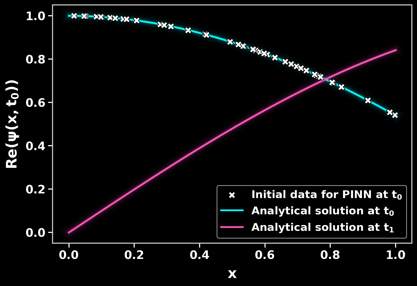
\[\psi(x, t) = e^{i(kx - \omega t)} \quad \text{with} \quad \omega = \frac{k^2}{2},\]with \(k = 1\) on the domain \(x \in [0, 1]\) and \(t \in [0, \pi]\). The plane wave is an exact solution, so we can easily check how well the network does.
1. Space and time in one go
Classical solvers usually march forward in time: They compute the solution at \(t + \Delta t\) from the solution at \(t\), step after step. In this first approach, we do something quite different. We treat time just like another spatial coordinate and solve the equation on the two-dimensional space-time domain \([x_l, x_r] \times [t_0, t_1]\) in one step. The network sees the whole history of the wave function at once. There are no time steps and no time discretisation at all. The initial condition is then simply a boundary condition on the \(t = t_0\) edge of this 2D domain.
Complex numbers
Neural networks usually work with real numbers, but the wave function is complex. The simplest fix is to let the network output two numbers: The real part and the imaginary part of \(\psi\). So our network \(\psi_\theta(x, t)\) takes two inputs \((x, t)\) and returns two outputs \((\mathrm{Re}\,\psi_\theta, \mathrm{Im}\,\psi_\theta)\). Here, \(\theta\) stands for all the weights of the network.
The residual
How do we tell the network that it should satisfy the Schrödinger equation? We move all terms to one side and define the residual
\[r_{\theta}(x, t) = \left(i \partial_t + \frac{1}{2} \partial_x^2\right)\psi_{\theta}(x, t).\]If \(\psi_\theta\) were the exact solution, the residual would be zero everywhere. Splitting it into real and imaginary parts, we get two real equations. Up to an overall sign, these are
\[\partial_t \mathrm{Re}\,\psi_\theta + \frac{1}{2}\partial_x^2 \mathrm{Im}\,\psi_\theta = 0 \qquad \partial_t \mathrm{Im}\,\psi_\theta - \frac{1}{2}\partial_x^2 \mathrm{Re}\,\psi_\theta = 0.\]TensorFlow’s GradientTape gives us the derivatives we need. For the second derivative in \(x\), we simply nest two gradient computations:
def compute_residual(model, xt):
    with tf.GradientTape(persistent=True) as tape:
        x, t = xt[:, 0:1], xt[:, 1:2]
        tape.watch(x)
        tape.watch(t)

        psi = model(tf.concat([x, t], axis=1))
        re, im = psi[:, 0], psi[:, 1]

        # First derivatives inside the tape so we can differentiate again
        re_x = tape.gradient(re, x)
        im_x = tape.gradient(im, x)

    re_t  = tape.gradient(re, t)
    im_t  = tape.gradient(im, t)
    re_xx = tape.gradient(re_x, x)
    im_xx = tape.gradient(im_x, x)
    del tape

    residual_re = re_t + 0.5 * im_xx
    residual_im = im_t - 0.5 * re_xx
    return tf.concat([residual_re, residual_im], axis=1)
The loss function
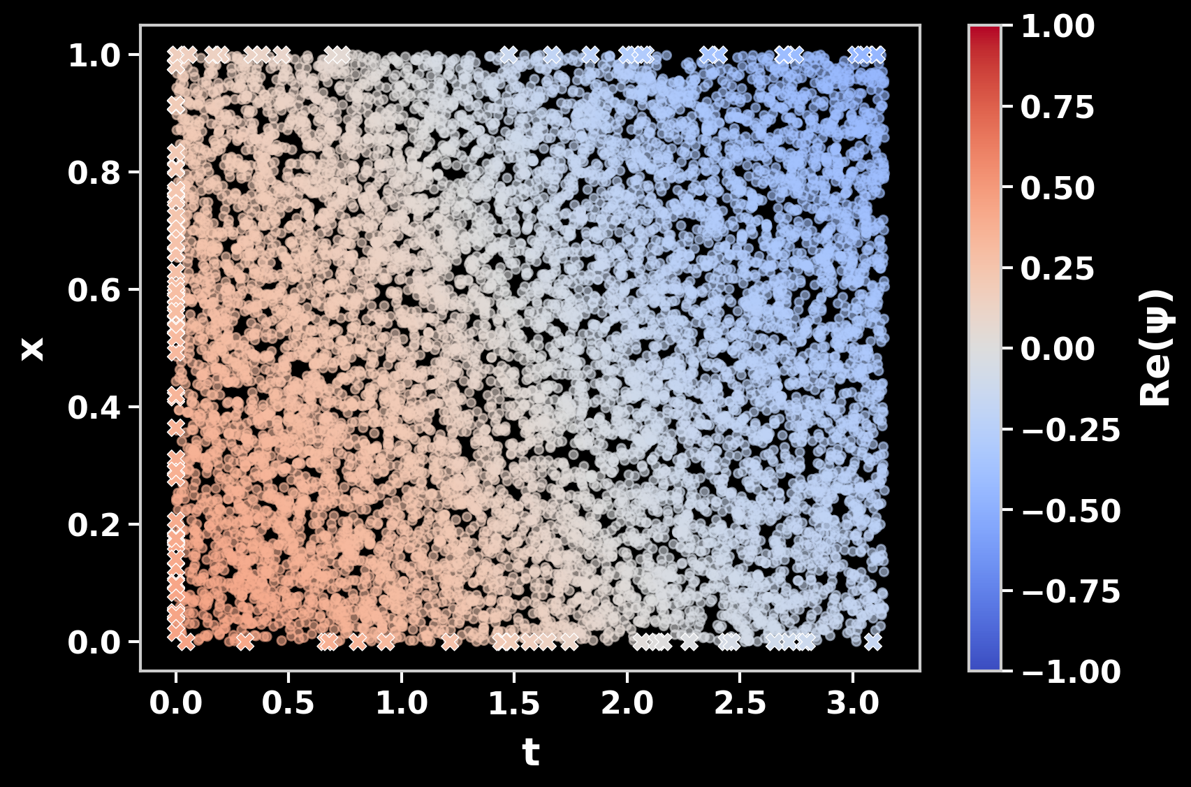
We evaluate the residual at many randomly chosen points inside the domain, the so-called collocation points. The loss function then consists of three terms:
\[\mathcal{L}(\theta) = \underbrace{\frac{1}{N_r}\sum_{j} |r_\theta(x_j, t_j)|^2}_{\text{PDE}} + \underbrace{\frac{1}{N_0}\sum_{j} |\psi_\theta(x_j, t_0) - \psi_0(x_j)|^2}_{\text{initial condition}} + \underbrace{\frac{1}{N_b}\sum_{j} |\psi_\theta(x_b, t_j) - \psi_b(t_j)|^2}_{\text{boundary conditions}}\]In code, this is just three mean squared errors added together:
def compute_loss(model, xt_collocation, xt_initial, psi_initial, xt_boundary, psi_boundary):
    loss  = tf.reduce_mean(tf.square(compute_residual(model, xt_collocation))) # PDE
    loss += tf.reduce_mean(tf.square(model(xt_initial)  - psi_initial))        # initial conditions
    loss += tf.reduce_mean(tf.square(model(xt_boundary) - psi_boundary))       # boundary conditions
    return loss
We use \(50\) points for the initial condition, \(50\) points on the boundaries and \(10000\) collocation points, all drawn from uniform distributions. Note how little information the network actually gets about the solution: Only \(100\) points on the edges of the space-time domain. Everything in between has to follow from the PDE.
The network
The network itself is a plain fully-connected feedforward network with \(4\) hidden layers of \(20\) neurons each and \(\tanh\) activations. We choose \(\tanh\) because it is smooth: We need to take second derivatives of the network, and activations like ReLU have vanishing second derivatives. The first layer rescales the inputs \((x, t)\) to \([-1, 1]\), which makes training easier.
def init_model(num_hidden_layers=4, num_neurons_per_layer=20):
    model = tf.keras.Sequential()
    model.add(tf.keras.Input(2))
    # Normalise input to [-1, 1] in all dimensions
    model.add(tf.keras.layers.Lambda(
        lambda x: 2.0 * (x - lower_bounds) / (upper_bounds - lower_bounds) - 1.0
    ))
    for _ in range(num_hidden_layers):
        model.add(tf.keras.layers.Dense(num_neurons_per_layer, activation="tanh", kernel_initializer="glorot_normal"))
    model.add(tf.keras.layers.Dense(2)) # real and imaginary part
    return model
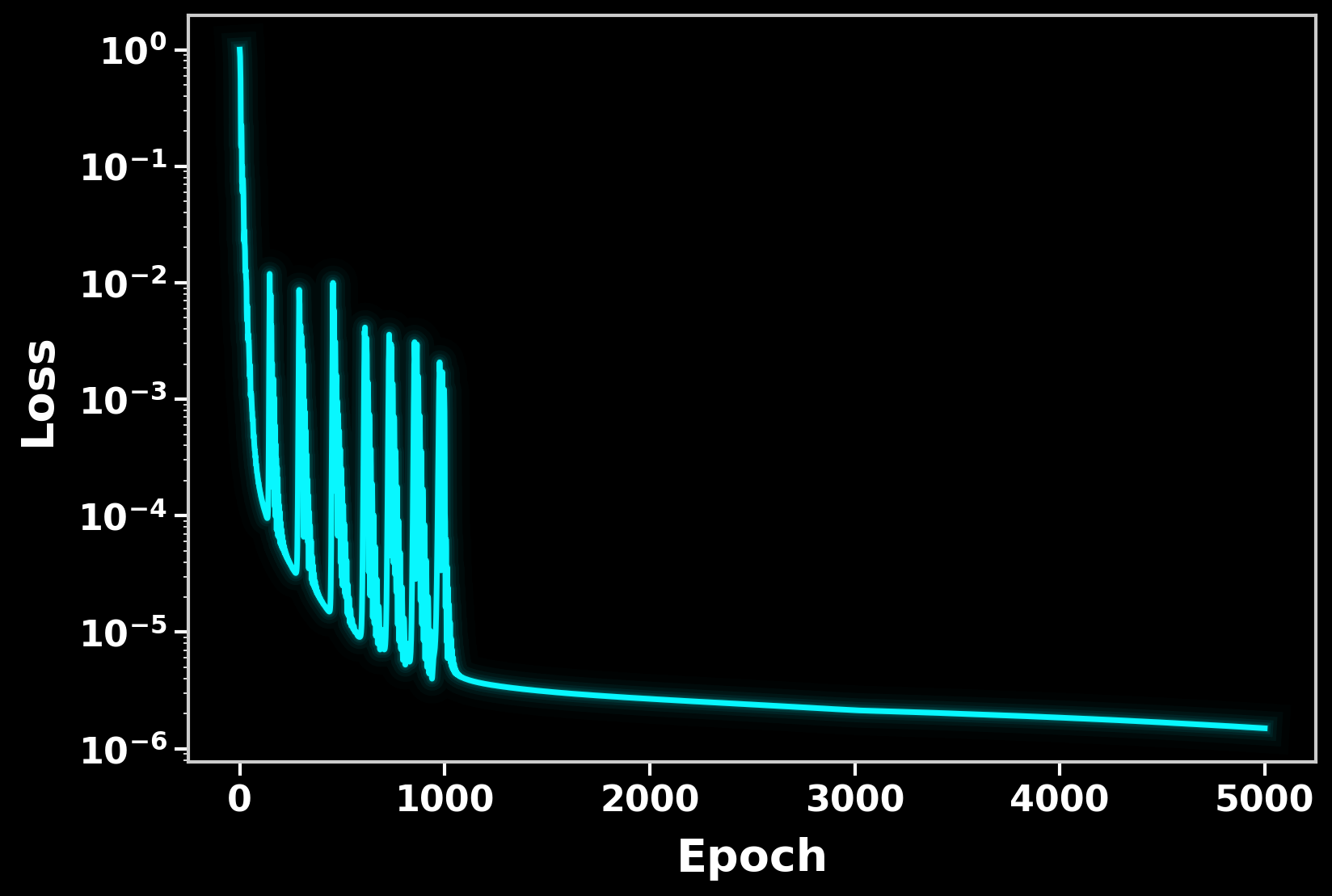
We train with the Adam optimiser for \(5000\) steps and decrease the learning rate from \(10^{-2}\) to \(10^{-3}\) after \(1000\) steps and to \(5 \cdot 10^{-4}\) after \(3000\) steps.
Results
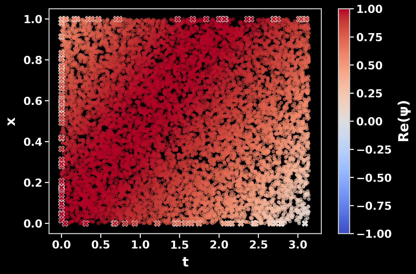
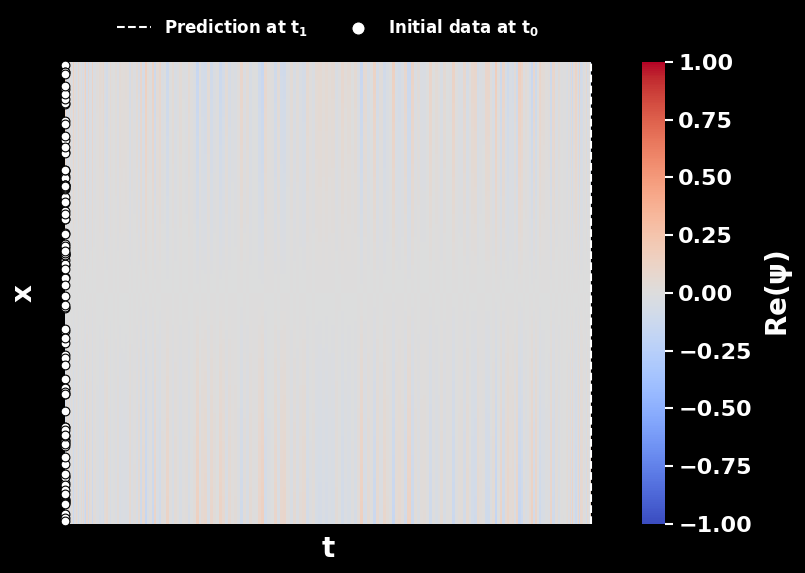
After training, the network reproduces the initial and boundary conditions. More interestingly, it also finds the correct plane wave inside the domain where it never saw any solution data: The \(L_1\) error on the collocation points is about \(5.9 \cdot 10^{-4}\). To make sure that the network did not simply memorise the collocation points, we also evaluate it on \(10000\) fresh test points. The error there is just as low, again about \(5.9 \cdot 10^{-4}\).
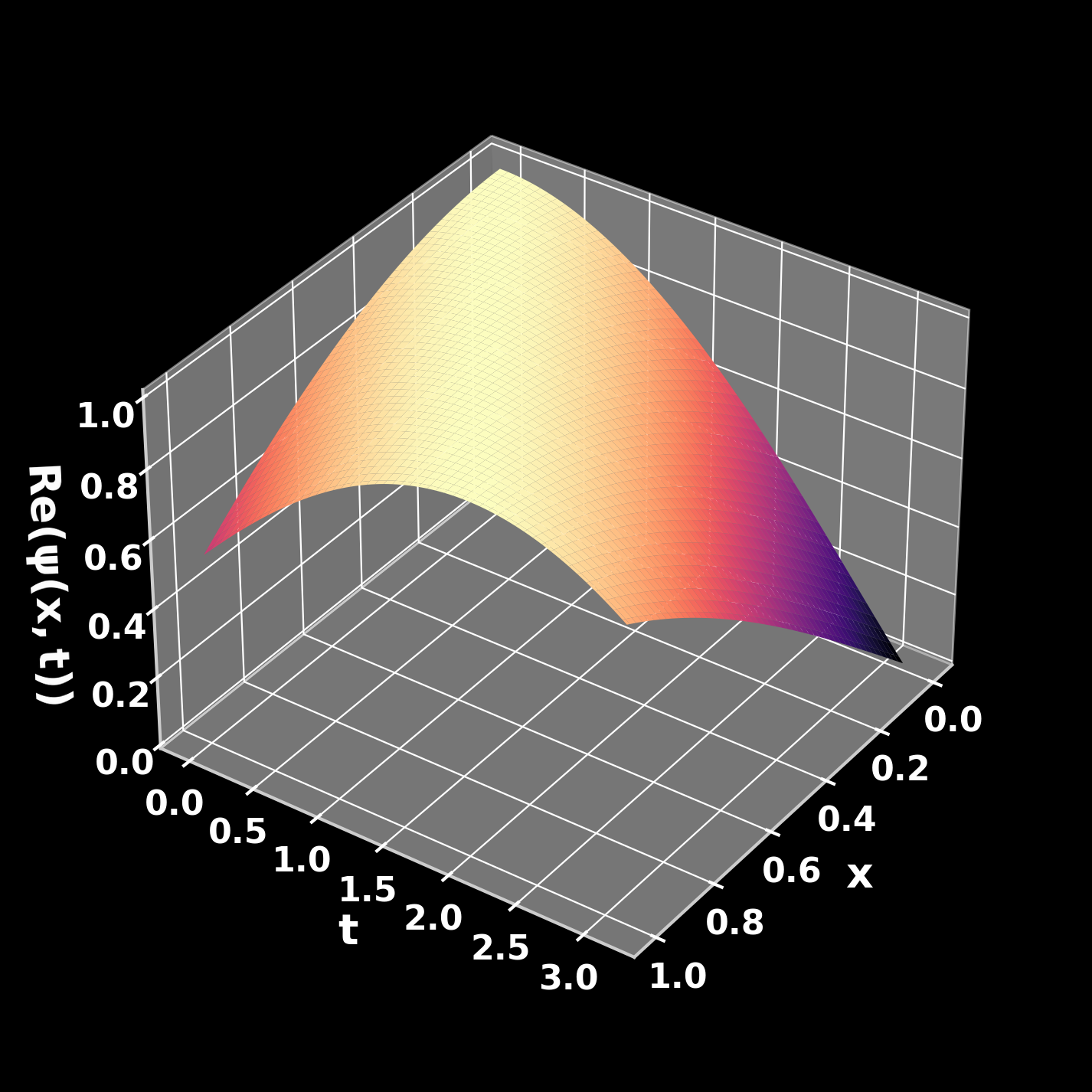
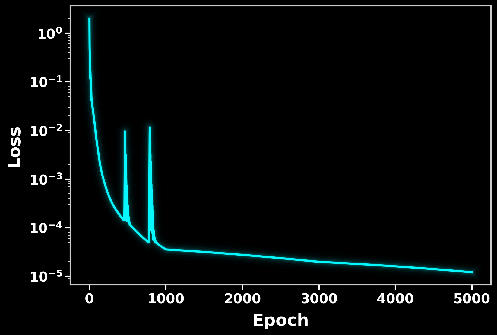
This is encouraging, but the plane wave is also about the friendliest problem one can think of: It is smooth, has a single frequency and the domain is short. Solving for all times at once also has a downside: The network has to represent the entire space-time solution, which becomes hard for long times or rapidly oscillating waves. In the next section, we therefore go back to a more classical idea and combine the network with an implicit time discretisation. The network then only has to learn the solution in space, while a Runge-Kutta scheme takes care of time.
2. One big time step
In their original paper, Raissi, Perdikaris and Karniadakis also proposed a second flavour of PINNs: Discrete time models. Here, we go back to the classical idea of time stepping, but with a twist. Instead of taking many small steps, we take a single, huge step of size \(\Delta t = t_1 - t_0 = \pi\) from the initial to the final time.
Implicit Runge-Kutta
To use a time stepping scheme, we write the Schrödinger equation as an ordinary differential equation in time:
\[\partial_t \psi = \mathcal{N}[\psi] \qquad \text{with} \qquad \mathcal{N}[\psi] = \frac{i}{2} \partial_x^2 \psi.\]An implicit Runge-Kutta (IRK) scheme with \(q\) stages then computes the solution \(\psi^{n+1}(x) = \psi(x, t_0 + \Delta t)\) from the initial condition \(\psi^n(x) = \psi(x, t_0)\) via
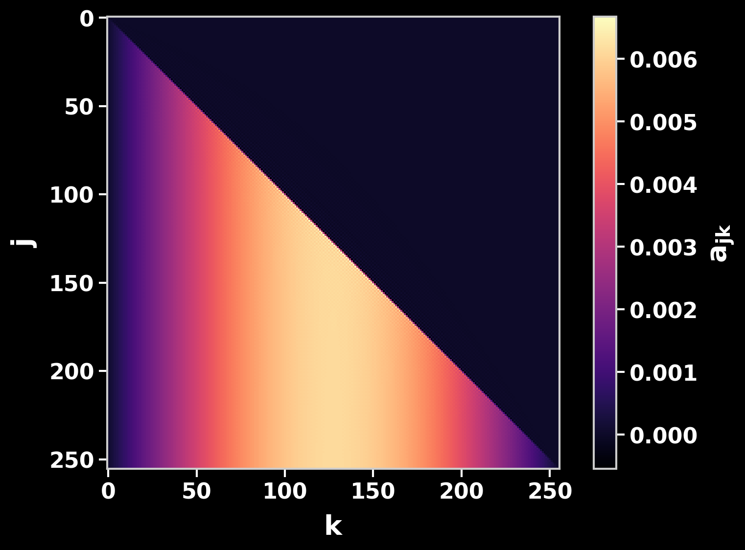
\[\psi^{n+c_j}(x) = \psi^n(x) + \Delta t \sum_{k=1}^q a_{jk} \mathcal{N}[\psi^{n+c_k}](x), \qquad j = 1, \dots, q\] \[\psi^{n+1}(x) = \psi^n(x) + \Delta t \sum_{k=1}^q b_k \mathcal{N}[\psi^{n+c_k}](x).\]The intermediate solutions \(\psi^{n+c_j}(x) = \psi(x, t_0 + c_j \Delta t)\) are called stages and the coefficients \(a_{jk}\), \(b_k\) and \(c_j\) make up the so-called Butcher tableau. Since the scheme is implicit, the stages appear on both sides of the equation. A classical solver would have to solve a large system of equations for all stages at once. This is where the network comes in: It simply learns the stages.
Why can we get away with a single time step? We use the Gauss-Legendre IRK scheme with \(q = 256\) stages from the PINN paper. Its temporal error scales like \(\mathcal{O}(\Delta t^{2q})\), which is far below machine precision even for our big time step. The accuracy of the result is therefore entirely limited by how well the network learns the stages.
The network
The network now only takes a single input, the position \(x\). Its output are all stages and the final solution at once:
\[\psi_\theta(x) = \left[\psi_\theta^{n+c_1}(x), \dots, \psi_\theta^{n+c_q}(x), \psi_\theta^{n+1}(x)\right].\]With real and imaginary parts, these are \(2(q+1) = 514\) outputs. Since the network has to represent a lot more information per input point, we make it a little wider and use \(50\) neurons in each of the \(4\) hidden layers:
def init_model(num_hidden_layers=4, num_neurons_per_layer=50):
    model = tf.keras.Sequential()
    model.add(tf.keras.Input(1)) # 1D input, time is handled by the IRK scheme
    # Normalise input to [-1, 1]
    model.add(tf.keras.layers.Lambda(lambda x: 2.0 * (x - xl) / (xr - xl) - 1.0))
    for _ in range(num_hidden_layers):
        model.add(tf.keras.layers.Dense(num_neurons_per_layer, activation="tanh", kernel_initializer="glorot_normal"))
    model.add(tf.keras.layers.Dense(2 * (q + 1))) # real and imaginary part for each of the q stages and for t1
    return model
The loss function
How do we train the network if we do not know the stages? We rearrange the IRK scheme such that the known initial condition is on the right-hand side:
\[\psi^n_j(x) = \psi^{n+c_j}_{\theta}(x) - \Delta t \sum_{k=1}^q a_{jk} \mathcal{N}[\psi^{n+c_k}_{\theta}](x) \overset{!}{=} \psi_0(x), \qquad j = 1, \dots, q\] \[\psi^n_{q+1}(x) = \psi^{n+1}_{\theta}(x) - \Delta t \sum_{k=1}^q b_k \mathcal{N}[\psi^{n+c_k}_{\theta}](x) \overset{!}{=} \psi_0(x).\]In words: If we take any of the \(q+1\) outputs and undo the time step, we should get back the initial condition. This is where the PDE enters. The loss function then consists of only two terms:
- The misfit between the \(q+1\) reconstructions \(\psi^n_j\) and the initial condition at \(N_0\) randomly drawn points \(x_j\).
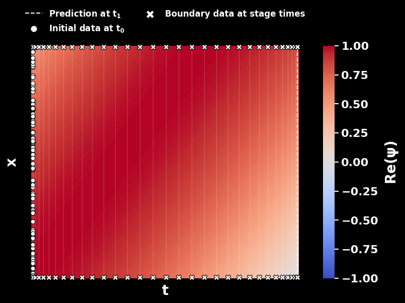
- The misfit between the network output and the boundary conditions at the \(q\) stage times and at \(t_1\).
There are no collocation points in time anymore. The dynamics are fully encoded in the IRK scheme. We use \(100\) points for the initial condition and, since the boundary is just two points in 1D, \(2(q+1)\) boundary values.
Derivatives of many outputs
To evaluate \(\mathcal{N}\), we need the second derivative of every output with respect to \(x\). This turns out to be trickier than in the continuous case. tape.gradient computes the gradient of the sum of all outputs, so the derivatives of our \(514\) outputs would be added up. Computing the full Jacobian would work, but is expensive.
Instead, we use a neat trick from Raissi’s implementation. We weight the outputs with a dummy vector \(u\) and compute the gradient
\[g(u) = \sum_k u_k \, \partial_x \psi_{\theta, k}(x).\]This expression is linear in \(u\), so differentiating it with respect to \(u_k\) gives us back the derivative of the \(k\)-th output \(\partial_x \psi_{\theta, k}(x)\). Doing this twice gives us the second derivatives. The IRK weights \(a_{jk}\) and \(b_k\) are stored as a single \((q+1) \times q\) matrix, so undoing the time step for all outputs is a single matrix product:
def compute_initial_reconstruction(model, x):
    dummy_1 = tf.ones((tf.shape(x)[0], 2*(q+1)), dtype=rtype)
    dummy_2 = tf.ones((tf.shape(x)[0], 2*(q+1)), dtype=rtype)

    # Nested tapes: each tape records the gradient computed by the tape inside of it
    with tf.GradientTape() as tape_dummy_2:
        tape_dummy_2.watch(dummy_2)
        with tf.GradientTape() as tape_x_2:
            tape_x_2.watch(x)
            with tf.GradientTape() as tape_dummy_1:
                tape_dummy_1.watch(dummy_1)
                with tf.GradientTape() as tape_x_1:
                    tape_x_1.watch(x)
                    psi_stages = model(x)
                g_1 = tape_x_1.gradient(psi_stages, x, output_gradients=dummy_1)
            psi_x = tape_dummy_1.gradient(g_1, dummy_1)
        g_2 = tape_x_2.gradient(psi_x, x, output_gradients=dummy_2)
    psi_xx = tape_dummy_2.gradient(g_2, dummy_2)

    # Split into real and imaginary parts, only the q stages enter N[psi]
    re    = get_real_stages(psi_stages)
    im    = get_imag_stages(psi_stages)
    re_xx = get_real_stages(psi_xx)[:, :q]
    im_xx = get_imag_stages(psi_xx)[:, :q]

    # N[psi] = i/2 psi_xx
    N_re = - 0.5 * im_xx
    N_im =   0.5 * re_xx

    # Undo the IRK step for all q+1 outputs
    re0 = re - dt * tf.matmul(N_re, irk_weights, transpose_b=True)
    im0 = im - dt * tf.matmul(N_im, irk_weights, transpose_b=True)
    return tf.concat([re0, im0], axis=1)
TensorFlow also offers forward-mode differentiation via tf.autodiff.ForwardAccumulator, which would be the natural choice here. Be careful though: Backpropagating through nested accumulators inside a tf.function silently yields wrong gradients with respect to the weights.
The loss function is then just two mean squared errors:
def compute_loss(model, x_initial, psi_initial_stages, x_boundary, psi_boundary):
    loss  = tf.reduce_mean(tf.square(compute_initial_reconstruction(model, x_initial) - psi_initial_stages)) # PDE and initial conditions
    loss += tf.reduce_mean(tf.square(model(x_boundary) - psi_boundary))                                      # boundary conditions
    return loss
We train with the same optimiser and learning rate schedule as before for \(5000\) steps.
Results
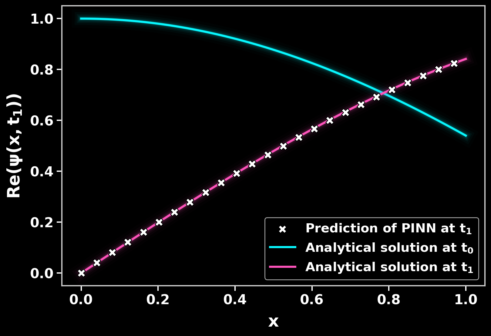
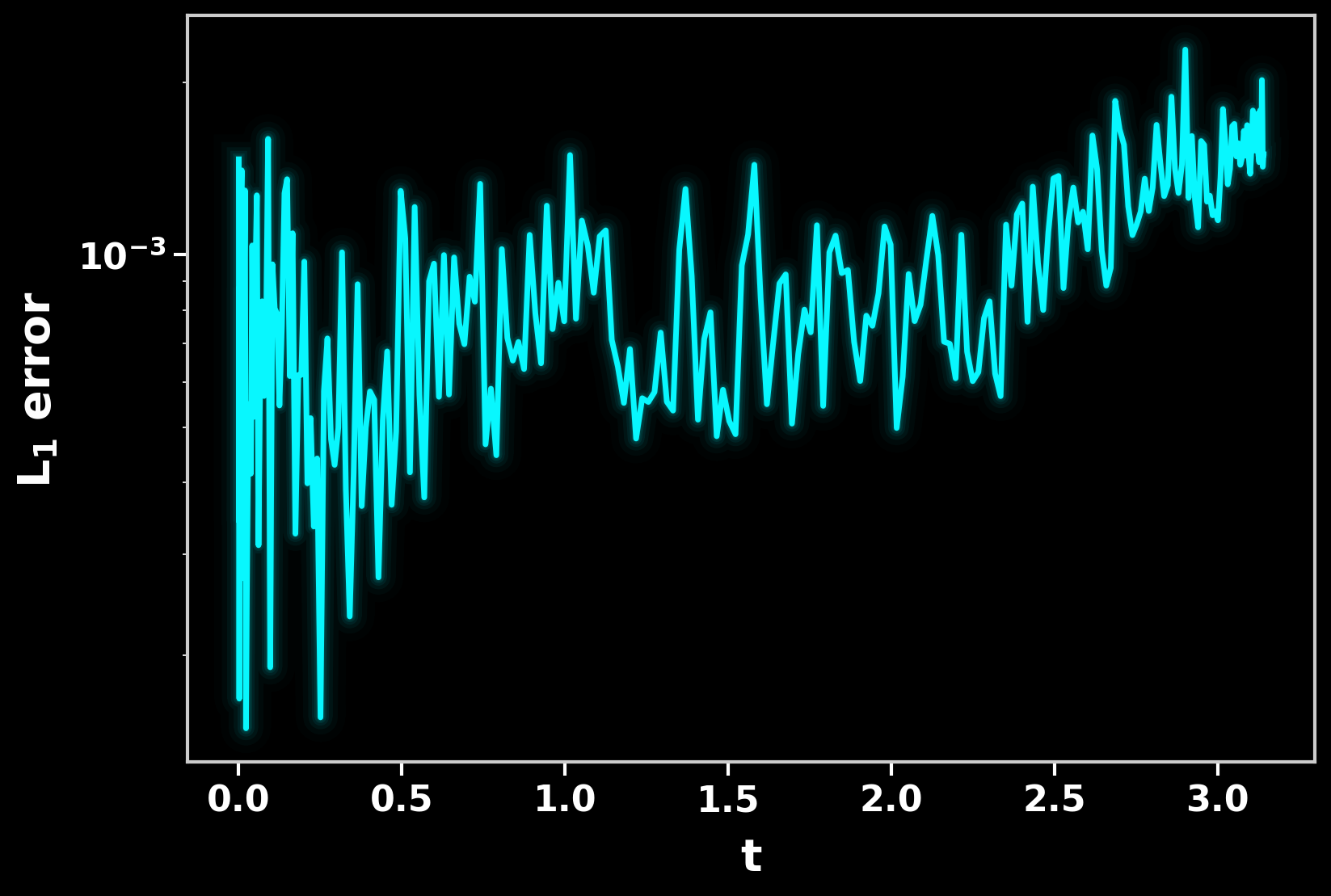
The network only ever saw data at \(t_0\) and on the boundary. Yet, after training, its prediction at the final time \(t_1\) lies right on top of the analytical solution, with an \(L_1\) error of about \(1.5 \cdot 10^{-3}\). As a by-product, we also get the solution at all \(q\) stage times inside the time step. Their errors are of the same size and grow slightly towards the end of the time step.
3. How good are PINNs really?
Both networks learnt the plane wave. But how good are they really? Let’s first compare them with each other and then with the classical solvers they are supposed to compete with.
Continuous vs. discrete time
Here is how both approaches do on the plane wave from above, trained for \(5000\) steps on the same CPU:
| Continuous time | Discrete time | |
|---|---|---|
| Training points | 10000 collocation + 50 initial + 50 boundary | 100 initial + 2 boundary |
| Network outputs | 2 | 514 |
| Training time | 398 s | 37 s |
| Final loss | \(1.2 \cdot 10^{-5}\) | \(1.5 \cdot 10^{-6}\) |
| \(L_1\) error | \(5.9 \cdot 10^{-4}\) (whole domain) | \(1.5 \cdot 10^{-3}\) (at \(t_1\)) |
| Mean density \(\vert\psi\vert^2\) (exact: 1) | 0.9999 | 0.996 |
The discrete time approach trains about \(11\) times faster, because the Runge-Kutta scheme replaces all the collocation points in time. Both errors are in the same ballpark. Note, however, that they are measured on different points: Over the whole space-time domain for the continuous and only at the final time for the discrete approach. Also note that neither network exactly conserves the total probability, something that good classical Schrödinger solvers do by construction.
PINNs vs. classical solvers
An error of \(10^{-3}\) sounds decent. To see whether it actually is, we pit both PINNs against three classical solvers: Finite differences of 4th and 6th order and a Fourier (FFT) solver. For a fair fight, the PINNs are ported to PyTorch with double precision and trained harder, with \(2000\) Adam steps followed by \(1500\) steps of the L-BFGS optimiser. The test problem is again a plane wave, this time with either \(2\) or \(16\) wavelengths in the domain. The wave travels a third of the domain before we measure the error.
We then increase the resolution \(N\): For the classical solvers, \(N\) is the number of grid points. For the PINNs, it is the number of training points per dimension. More points should mean a smaller error.
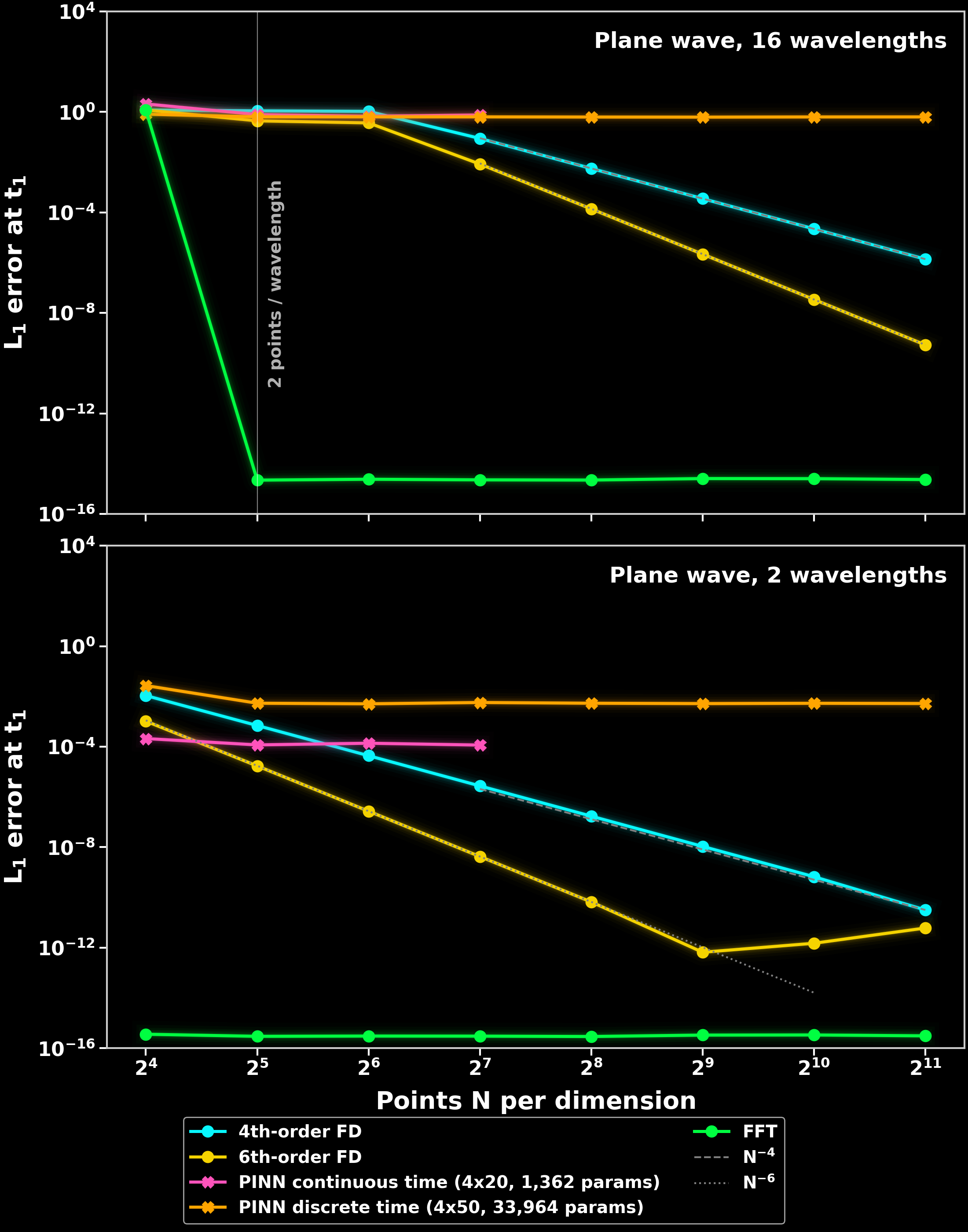
The result is sobering:
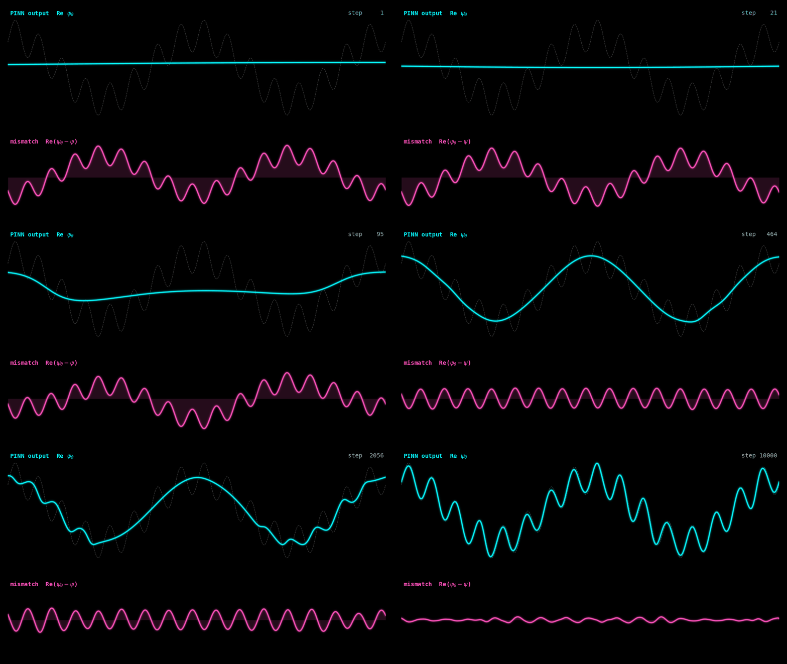
- 16 wavelengths: Neither PINN learns the solution at any resolution, with errors of order one. At the same time, 4th-order finite differences already reach \(10^{-6}\). The culprit is the so-called spectral bias of neural networks that you already saw in action in Figure 1: Networks like ours learn smooth, slowly varying functions quickly and rapid oscillations very, very slowly. Unfortunately, rapid oscillations are exactly what makes the Schrödinger equation hard.
- 2 wavelengths: Both PINNs learn the solution, but their errors stay flat at about \(10^{-4}\) (continuous) and \(5 \cdot 10^{-3}\) (discrete), no matter how many points we give them. The final loss is also the same for every \(N\). So the bottleneck is not the data, but the optimiser that cannot push the loss any lower.
The classical solvers, on the other hand, behave exactly as the textbook says: Their errors fall steadily with \(N\) until they hit round-off. The FFT solver is exact to machine precision as soon as it has two points per wavelength.
Maybe the networks are simply too small? Figure 14 shows what happens when we make them wider.
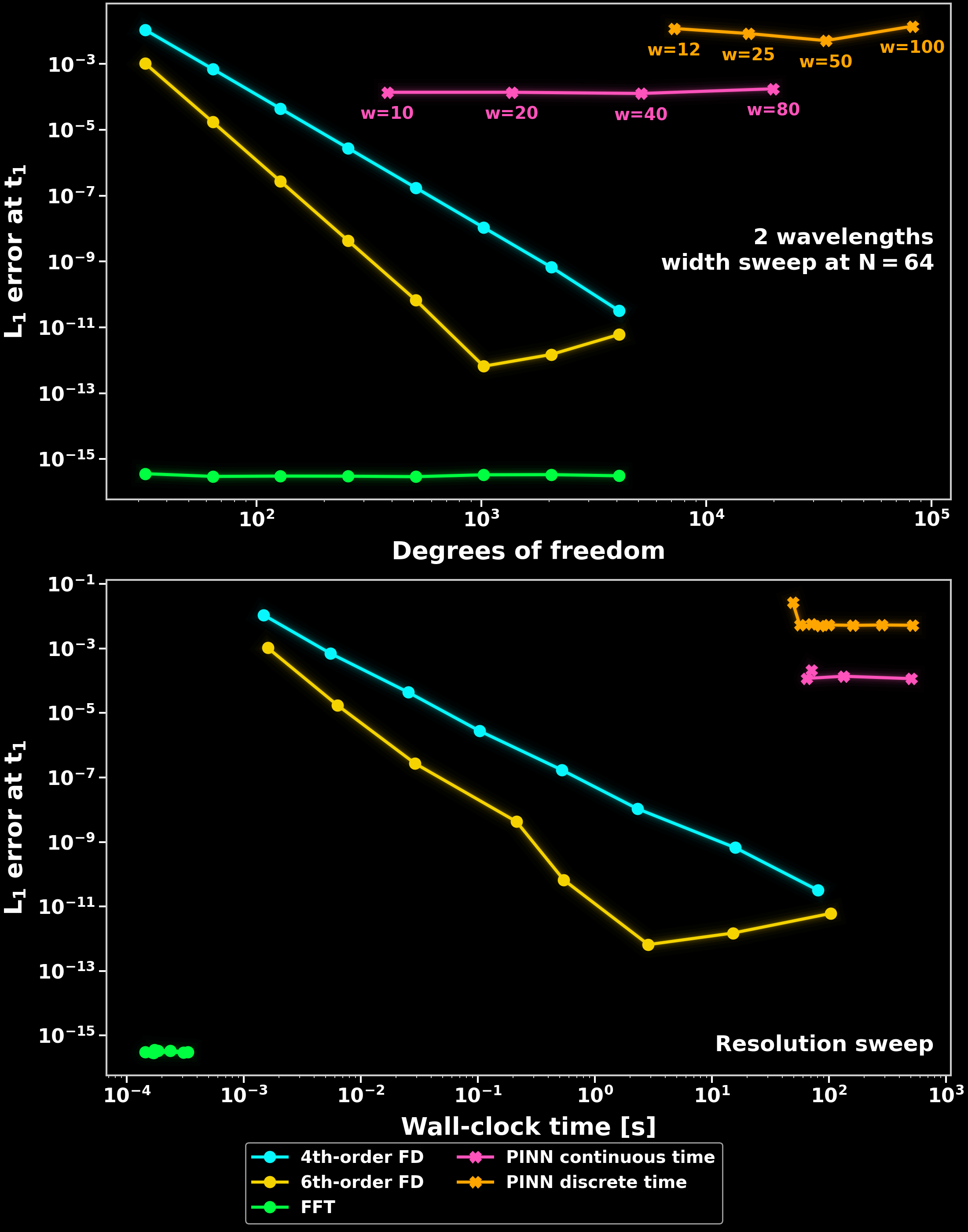
Network size barely matters. Across networks from a few hundred to \(82000\) parameters, the continuous time PINN stays stuck at about \(1.5 \cdot 10^{-4}\) and the discrete one even gets worse when it gets wider. At the same number of degrees of freedom, finite differences are \(5\) to \(10\) orders of magnitude more accurate and about \(1000\) times faster. Between the two PINNs, the continuous one comes out on top: It is about \(40\) times more accurate with \(25\) times fewer parameters. Most parameters of the discrete network sit in its huge output layer with \(514\) outputs. Keep in mind that every point is a single training run, so the PINN values would scatter by roughly a factor of two for different random seeds.
Taking huge time steps
There is one more argument for the discrete time PINN: It takes a single, huge time step, while explicit classical solvers have to take many tiny ones to remain stable. So does it win when the time step becomes large?
To find out, we take one time step of size \(\Delta t\) for a plane wave in the periodic potential \(V(x) = 20 \cos(2 \pi x)\). Without a potential, the Fourier solver would be exact for any time step, so the potential is what makes the problem hard, just as in the Schrödinger-Poisson equation. We increase the step size from \(\omega \Delta t = 1\), i.e. a sixth of an oscillation period, to \(\omega \Delta t = 128\), i.e. about \(20\) periods. We compare the PINNs with two classical solvers that can take large steps, split-step Fourier and Crank-Nicolson, and with the implicit Runge-Kutta scheme solved exactly. The latter is what a perfectly trained discrete time PINN would achieve. We also test an improved discrete time PINN that adapts the number of stages \(q\) to the step size.
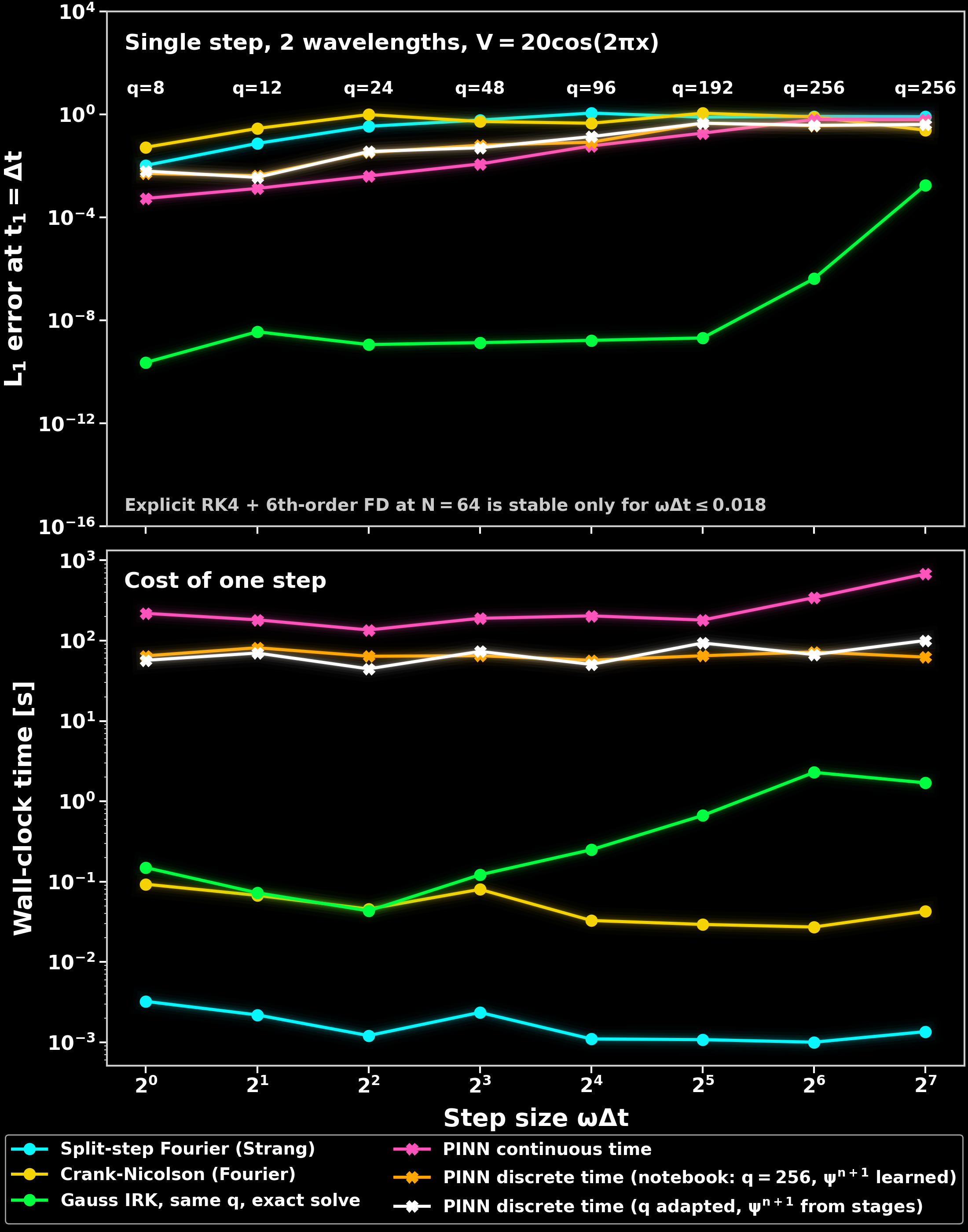
The exact IRK solve shows that the idea works in principle: With enough stages, a single step is accurate to about \(10^{-9}\) up to \(\omega \Delta t = 32\), i.e. across five oscillation periods. Only when even \(256\) stages are no longer enough does its error rise. The PINNs, however, do not get anywhere near that. Their errors start at \(10^{-3}\) to \(10^{-2}\) for small steps and grow to order one for large steps. Adapting the number of stages barely helps. The problem is not the Runge-Kutta scheme, but that training cannot find the stages accurately.
Split-step Fourier and Crank-Nicolson do not do well with a single huge step either. But they do not have to take one: A split-step Fourier step takes about a millisecond, while training a PINN for one step takes one to ten minutes. In the time it takes to train a single PINN, a classical solver can take tens of thousands of small, accurate steps. So even in the discipline that was supposed to be their strength, the PINNs lose.
Conclusion
So, should you throw away your Schrödinger solver? Not yet. On a simple, linear forward problem like ours, plain PINNs lose to classical solvers in every respect: They are less accurate, much slower, do not get better with more data or bigger networks and fail completely once the solution oscillates rapidly. That does not mean that PINNs are useless. They shine where classical solvers struggle, for instance when we want to combine the equations with measured data or infer unknown parameters. But if your worry is resolving the tiny wavelengths of the Schrödinger equation, PINNs in their plain form will not take it away. In the next posts, we will look at other algorithms that try to do better.