Computers learning Bomberman Pt. 1: Tabular Q-learning
In today's post, we use the tabular Q-learning algorithm to learn how to play the Bomberman clone BombeRLe designed for reinforcement learning. You may find the accompanying Python code on GitHub. For an introduction to tabular Q-learning, please refer to the Tic-Tac-Toe series.
BombeRLe: Game Mechanics Explained
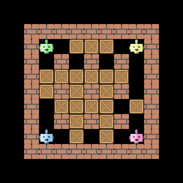
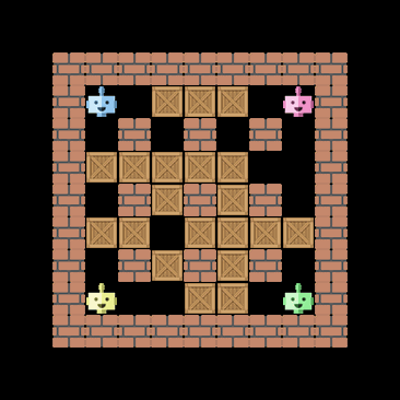
In BombeRLe, up to four agents compete by collecting coins and placing bombs to destroy crates and eliminate enemies. The goal of the game is to collect as many coins and kill as many enemies as possible.
- The game is turn-based and each agent has 6 possible actions: Move up, right, down, left, place a bomb and wait
- Agents act in random order. This means that depending on who moves first walking into another player moving away will sometimes result in waiting, sometimes in moving.
- Walking into an obstacle (wall, bomb, crate) results in waiting instead but an agent can stand on its own bomb after placing it.
- Agents blow up crates using bombs and collect coins by walking through them.
- Every player has one life and dies immediately when stepping into an explosion. If an agent kills another player and dies at the same time, this counts as kill.
- If an agent kills itself, it does not lose points and no other agent gains points.
- Explosions are not stopped by crates. They pass through bombs but do not ignite them.
- Players can place only one bomb at a time. The timeline of a bomb is detailed in the table below and depicted in Figure 1.
| Frame | State | Description |
|---|---|---|
| 1 | Agent drops the bomb | New bomb with time to explosion t = 4 |
| 2 | Bomb ticking | Bomb timer counts down to t = 3 |
| 3 | Bomb ticking | Bomb timer counts down to t = 2 |
| 4 | Bomb ticking | Bomb timer counts down to t = 1 |
| 5 | Bomb explodes | Explosion at t = 0, affecting 3 tiles |
| 6 | Explosion remains | Explosion lingers for 1 frame |
| 7+ | Agent can place a new bomb | Harmless smoke remains for 2 frames |
Your best friend for efficient training: Hyperparameters
The game allows for a number of settings that can be found in settings.py
- Coins: 1 point per coin
- Kills: 5 points per enemy killed
- Crate density: Default is
0.75, can be adjusted by scenario - Number of coins: Default is
9, can be adjusted by scenario - Board size: My default is
9x9(including walls) - Bombs: Explode in the
4th frame after being dropped, explosion affects a radius of3fields and is present for2frames
A good state representation for tabular Q-learning should be small
Tabular Q-learning requires the game to be represented through a finite number of states. Bomberman is a discrete, turn-based game, hence, perfectly suitable for tabular Q-learning. But you may ask whether we can simply enumerate all possible board states and put them into the table. It turns out that this is unfeasible: assuming a small \(9\times9\) board with \(7\times7−9 = 40\) free fields that can either be free, occupied by a crate, a coin, an agent, or an explosion gives roughly \(4^{40} = 2^{80}\approx 10^{24}\) states. And this does not even account for bomb availability, explosion timers, or bomb timers. A Q-table for six possible actions (UP, RIGHT, DOWN, LEFT, BOMB, WAIT), using 4-byte floating point numbers, would require around \(10^{10}\) petabytes. Beyond memory requirements, trainability is another important consideration: a more granular state representation captures more nuances of the game, but requires more training data. Unlike DQN, tabular Q-learning does not extrapolate. So, the agent will necessarily fail in states it has not seen before. Therefore, we need to find a simplified representation of the game state. The upper size limit will roughly be a 32-bit representation, corresponding to a 100 GB-table if all states are populated. So, you should aim for less than 30 bits in most cases. After some experimentation, I settled for the following 18-bit representation:
| Bits | Field | Description |
|---|---|---|
| 0–2 | Neighbour (UP) | 3-bit code for object in UP direction: EMPTY, WALL, COIN, CRATE, ENEMY, BOMB, DANGER |
| 3–5 | Neighbour (RIGHT) | 3-bit code for object in RIGHT direction |
| 6–8 | Neighbour (DOWN) | 3-bit code for object in DOWN direction |
| 9–11 | Neighbour (LEFT) | 3-bit code for object in LEFT direction |
| 12–13 | Direction to nearest object | 2-bit code: 00 = UP, 01 = RIGHT, 10 = DOWN, 11 = LEFT |
| 14–15 | Type of nearest object | 2-bit code: 00 = NONE, 01 = ENEMY, 10 = CRATE, 11 = COIN |
| 16 | Action safe: BOMB | 1 = safe, 0 = unsafe |
| 17 | Action safe: WAIT | 1 = safe, 0 = unsafe |
The four 3-bit fields summarize the nearest tile in each direction:
- WALL, CRATE, BOMB, ENEMY, COIN, EMPTY: Encode the board as seen in the current time step (no future prediction).
- DANGER: Stepping onto that tile now makes survival impossible given the current bombs and blast timers.
- one unused state that could be used to distinguish bombs with different timers, enemies with and without bombs etc.
I define an action as safe if executing that move still allows the agent to survive given the current board state. That is, there exists at least one follow-up move or WAIT that avoids all dangers until all bombs have exploded. This gives the agent the basic capacity to avoid walking into flames, trapping itself with its own bombs, or failing to escape in time. It does not protect against being intentionally trapped by another agent or bombs being set off by other bombs, for instance. So, this representation will not lead to an ideal agent. But in practice, the trained agent should no longer needlessly kill itself. Furthermore, it should reliably dodge explosions, break crates, collect coins, and occasionally kill another agent if it gets lucky. It will, however, still lose to a smart opponent that traps it in tunnels, for instance.
These first twelve bits of the 18-bit representation allow the agent to perceive its immediate surroundings and assess dangerous situations to some extent. However, the agent still lacks any sense of the wider game board. To remedy this, I introduce 4 more bits that encode the direction and type of the nearest object of interest. This encoding implies the agent can only pursue a single object of interest at a time. It will not be aware of, say, two coins at equal distance.
The code runs a breadth-first search (BFS) to locate the nearest coins, crates, and agents. We guide the agent toward the nearest crate if it is within three steps, then the nearest agent not separated by walls or crates if it is within three steps. If there is none, we guide the agent towards the nearest walkable coin. Failing that, the nearest walkable crate. If none of those are available - the board has been blown up and all coints are collected - the agent is guided towards the closest remaining enemy. At first, I thought that guiding the agent towards the closest enemy available is a good strategy. But that led it to ignore many coins and crates on the way. Since coins are essential to high scores, it turns out that prioritising coins over crates and agents is a good strategy.
Once the agent knows where it can go, two final choices remain: Should the agent wait or place a bomb? To answer this question, I added 2 more bits indicating whether waiting and bombs are safe or unsafe using the same danger logic as before. Waiting is safe if no bombs can kill the agent in its current position; placing a bomb is safe if waiting is safe and the agent has an escape route before the bomb goes off.
This representation consumes 18 bits in total, translating to \(2^{18} = 262,144\) possible states. A Q-table with 6 actions and 4-byte floats would then require about \(2^{18} * 6 * 4 \text{ bytes} = 6,291,456 \text{ bytes} \approx 6 \text{ megabytes}\).
However, since many states are never visited during training, I store the Q-table as a hash table (i.e. a Python dictionary). This trades a slight performance penalty on lookup for a reduction in memory use, down to just a few hundred kilobytes for a typical training run.
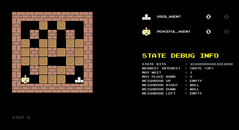
The animation shown in Figure 2 illustrates this encoding in practice. It shows the raw bit string, its division into the logical components described above, and the corresponding decoded categories. I found this reverse translation very helpful for debugging the encoding and would recommend building such a debug screen when designing state representations.
Another debugging step is to build a rule-based agent based on your state representation. With the 18-bit representation as input, we can easily define some sensible rules:
- move towards the object of interest if possible
- drop bombs when next to enemies and crates
- do not take dangerous actions
- choose randomly among the remaining actions By observing such a rule-based agent play a small number of rounds, you can quickly spot bugs in your encoding. For instance, I realised that bombs do not trigger other bombs. In addition, it turns out that this rule-based agent plays fairly well. The tabular Q-agent will have to beat it to prove its worth.
A good reward system helps even when in-game rewards are scarce
Ideally, our reward system should mirror the game’s reward system and maintain the same relative rewards for collecting coins and killing players. However, in practice rewards are sparse, especially when the player has to blow up crates to find coins and plays against strong opponents. Therefore, I introduce additional rewards that help the agent learn to explore the game.
I mirror the in-game rewards with the reward values for COIN_COLLECTED and KILLED_OPPONENT. Additionally, the player is rewarded for dropping bombs and destroying crates to incentivise aggressive play. It gets punished for killing itself and getting killed but killing itself is slightly less negative. I later realised that the game hands out both the GOT_KILLED and KILLED_SELF rewards when the player commits suicide. So, this reward system actually strongly disincentivises suicide (-1.90). In principle, suicide can be better than getting killed and should perhaps even receive a positive reward. This is because there is no penalty for suicide whereas getting killed means that the enemy is getting points. In practice, the agent is still fairly suicidal even with the current reward system.
| Event | Reward | Description |
|---|---|---|
| COIN_COLLECTED | +0.20 | Agent collected a coin |
| KILLED_OPPONENT | +1.00 | Agent killed another agent |
| CRATE_DESTROYED | +0.10 | Agent destroyed a crate |
| BOMB_DROPPED | +0.02 | Agent dropped a bomb |
| KILLED_SELF | −0.90 | Agent killed itself |
| GOT_KILLED | −1.00 | Agent got killed by opponent |
| WAITED | −0.02 | Agent performed a WAIT action |
| INVALID_ACTION | −0.02 | Agent performed an invalid action |
Faster Training Through Demonstration
For the Tic-Tac-Toe agent, I simply let the agent play games and updated the Q-table on the fly. This time, I would like to accelerate training to enable a more thorough sweep of the hyperparameter space.
One key opportunity I overlooked in Tic-Tac-Toe was the availability of a near-perfect demonstrator: the Minimax agent. Similarly, in the case of BombeRLe, the developers kindly provide a rule-based agent that performs reasonably well. We can leverage it to speed up training significantly by pre-recording a large number of transitions and using them to pre-train the Q-table. This is called offline learning. In contrast, sampling training data from the agent while it is learning is called online learning.
Offline learning with a demonstrator allows the agent to explore useful game states right from the beginning. In practice, I record 50,000 episodes from the demonstrator and use them to update the Q-table before performing any training or evaluation. I also enable exploration for the demonstrator - it also takes random actions so that the demonstration data is more diverse. In the first episode, the demonstrator only takes random actions. This exploration decays with a factor \(\epsilon\) to a floor value, just like in online training. I have not actually verified whether that is necessary but given that we need to extensively explore the state space for offline Q-training to work, I am confident it is not a bad idea.
The advantage of offline learning: While a full training run with online updates can take an hour, updating the Q-table with 50,000 recorded episodes takes a couple of minutes. This enables rapid experimentation across different hyperparameter configurations.
The key speed gain comes from the fact that we only need to compute the computationally expensive game state to integer state embedding once. These embeddings can then be reused across multiple hyperparameter runs. The training process itself is reduced to an iteration over transitions and matrix updates.
What settings for the training?
Throughout training, I keep the hyperparameters fixed to the values given below:
- Discount factor (γ): 0.8
- Constant Learning rate (α): 1e-3
- Initial Q-values: 0.0
I did experiment with an adaptive learning rate \(\alpha = lr_0 / (1 + N_{\text{visits}}\text{(state, action)}).\) This formulation decreases the learning rate as the agent gathers more experience with a specific (state, action) pair. Early in training, updates are larger and help the agent adapt quickly. Later, as visit counts increase, the learning rate decays, stabilising the learned Q-values and reducing variance. This strategy can help avoid overfitting to noisy or rare transitions and provides better convergence guarantees.
Yet, I performed a hyperparameter search using optuna and did not find that the adaptive learning rate improved performance for the agent presented here, but I might have made a mistake, so you should definitely try it out. You can also change the denominator to a non-linear function or introduce a floor.
Money, money, money
We start training in a simplified environment without enemies or crates, a small \(9\times9\) board and coins everywhere - the scenario baptised coin-heaven by the game.
How should we initialise the Q-table? Since we’re using offline learning (based on the demonstrator), the agent may not explore all available states. Initialising Q-values to a high value would encourage the agent to explore, but also risks overestimating actions not demonstrated. Instead, I found that initialising the Q-values to zero or a negative value is better. My understanding is that a pessimistic agent better learns to value good actions based on demonstrator input.
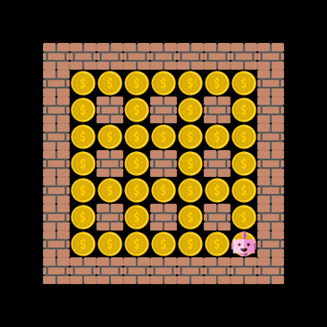
The agent reliably collects all coins. However, its path is not fully optimised: it always moves toward one of the nearest coins but does not plan multi-step routes that could reduce total steps. This is due to the BFS algorithm, which only targets the next closest coin and ignores multi-coin path efficiency.
Additionally, the agent’s behavior reflects a design choice: the pathfinding algorithm always prefers the closest object of interest following a fixed order of directions.
Blowing up crates for fun
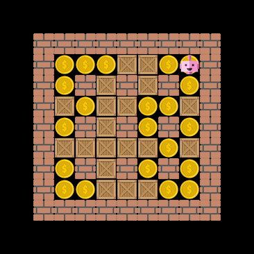
Next, we train on a more complex board configuration with crates but still without enemies - a scenario baptised loot-crate by the game. The learns how to successfully blow up crates. I also experimented with a 16-bit representation dropping the type of the object of interest to save 2 bits. However, the agent would get caught in infinite up-down loops or just wait. My interpretation is that the agent benefits from being able to distinguish between coins and crates (even though I am not 100% sure why this should matter in tabular Q-learning). My takeaway is that the representation matters more that I thought at first. More generally, I tend to suspect hyperparameters when machine learning algorithms underperform, but for tabular Q-learning and Bomberman the quality of the state representation seemed to be much more important than everything else once the algorithm was up and running.
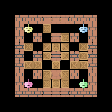
It’s time for war - training the allstar
In the final training phase, I simulate a full game in the classic scenario with multiple agents:
- Two rule-based agents
- One peaceful agent that moves randomly and doesn’t place bombs
- One tabular Q-learning agent
The tabular Q-agent after 50,000 training episodes, referred to as allstar hereafter, plays fairly well and tends to achieve higher scores than the rule-based agents.
How to understand these results?
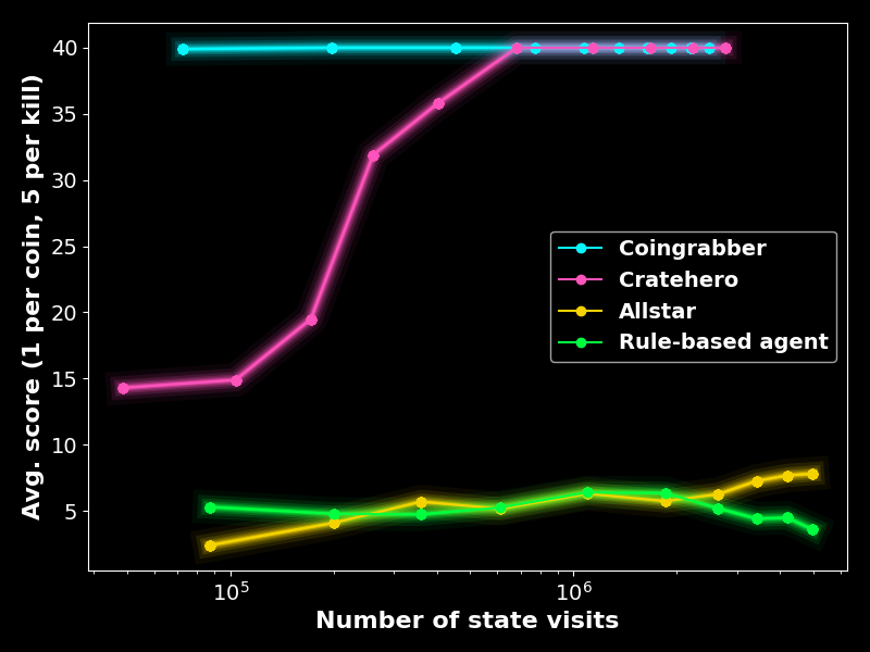
Training these agents, I wondered which metrics we could best use to assess the training process. An obvious choice is to check the scores the agents achieve. Figure 7 shows the scores of the three agents throughout the training: The coin grabber in the coin-heaven scenario (40 coins, no crates, no enemies), the crate hero in the loot-crate scenario (40 coins, crates, no enemies) and the allstar in the classic scenario (9 coins, crates, 3 enemies) as well as the rule-based agent playing agains the tabular Q-agent in the classic scenario for reference. The croin grabber and crate hero quickly converge to optimal policies. The allstar achieves higher scores than the rule-based agents but seems to be still improving.
Next, we assess the performance of the allstar by studying the averaged results of 1,000 games between the allstar agent, a rule-based agent, a peaceful agent and the rule-based agent using the simplified state representation - the representator - discussed in Figure 3. I checked that 1,000 games provide sufficient statistics for reproducible results.
| Category | allstar | peaceful_agent | rule_based_agent | representator |
|---|---|---|---|---|
| bombs | 18 | 0 | 8 | 19 |
| coins | 3.5 | 0.33 | 2.1 | 3 |
| crates | 6.5 | 0 | 6.3 | 8.1 |
| invalid | 2.1 | 18 | 4.7 | 3.4 |
| kills | 0.57 | 0 | 0.48 | 0.62 |
| moves | 1.3e+02 | 14 | 69 | 1.3e+02 |
| score | 6.3 | 0.33 | 4.5 | 6.1 |
| steps | 1.5e+02 | 33 | 84 | 1.5e+02 |
| suicides | 0.61 | 0 | 0.34 | 0.52 |
| time | 0.08 | 0.00099 | 0.04 | 0.061 |
In general, the allstar agent places more bombs, collects more coins, destroys the same number of crates, makes fewer invalid moves, is a better killer, moves more, achieves 50% higher scores and is more suicidal than the inbuilt rule-based agent. What is more interesting is the comparison with the representator: it turns out that the rule-based agent based on the simplified state representation achieves similar scores as the allstar. I am not sure whether I should be disappointed but I guess you reap what you sow: Given that the features were handcrafted with a certain purpose in mind and mostly show the agent its immediate surroundings, it should not be too surprising that the Q-learning process mostly consists in discovering the meaning of the features. The allstar is slightly more suicidal, collects fewer crates and achieves fewer kills but collects more coins than the representator.
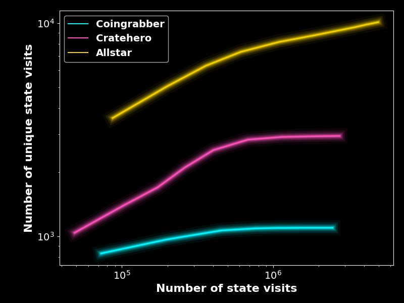
Let us focus on the allstar agent’s training process next. It is insightful to check how many unique states are visited during trainin. Figure 8 shows that the training data for both the coin grabber and the crate hero does not contain new unique states after around 500,000 states. In contrast, the allstar training set contains new states until the end of the training, suggesting that the training set might benefit from being larger. I did, however, test training with 250,000 episodes and the agent’s performance did not improve anymore, suggesting that the bottleneck is elsewhere.
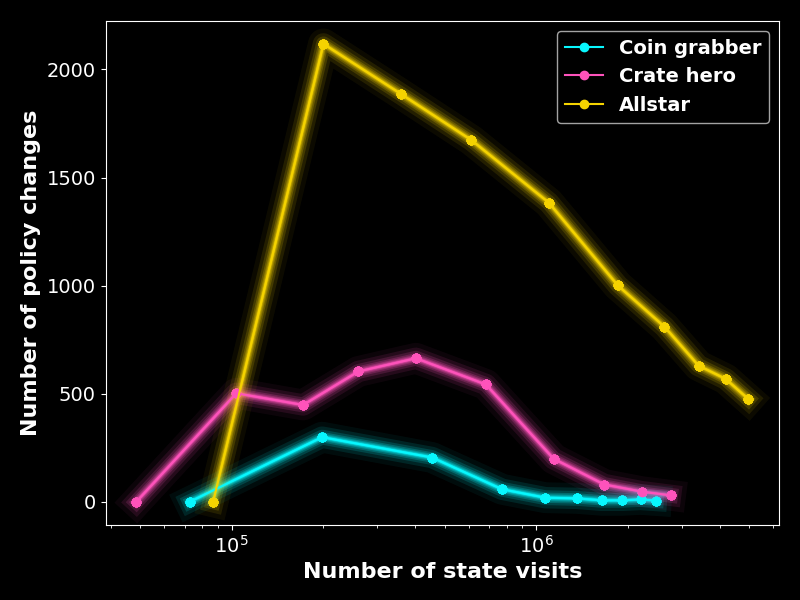
Going beyond that, we could look at how the Q-values or the number of state visits evolves during training but I personally find these metrics hard to interpret. I was hoping to gain insights from studying the Bellmann time difference error distribution over time, but to be honest, I was not able to tell whether the training had converged by looking at the time difference errors even though they are probably the closest counterpart of a training loss in tabular Q-learning. What did turn out to be interesting is to look at the number of policy changes, that is, that number of states where the best action has changed - over the course of the training. Figure 9 shows these policy changes and highlights that the crate hero’s and allstar’s policy’s have not completely converged after 50,000 episodes of offline training.
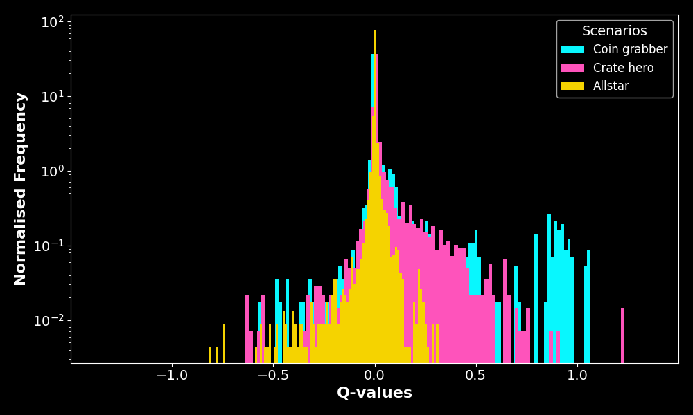
You may find some more plots of different distributions such as the Q-value distribution shown in Figure 10 in the accompanying notebooks. It is interesting to see that the distributions are centered around \(Q = 0\). Using optuna, I also found that \(Q_0 = 0\) is the best initialisation for the Q-table with this reward system.
Conclusion
In this post, we trained a tabular Q-learning algorithm to play a Bomberman clone. The tabular Q-learning algorithm worked well and the final agent has abundant potential for improvement - more offline training, online training, a better state representation etc. However, I personally find that there is too much handcrafting involved in developing a good state representation - developing a good tabular Q-agent seems to be almost as much work as developing a good rule-based agent. Therefore, we turn towards DQN and convolutional networks for automatically learning good features in the next post.