Computers learning Bomberman Pt. 2: Deep Q-learning
In today's post, we use the Deep Q-learning algorithm with convolutional neural networks to learn how to play the Bomberman clone BombeRLe designed for reinforcement learning. You may find the accompanying Python code on GitHub. For an introduction to Deep Q-learning, please refer to the Tic-Tac-Toe series on this blog.
How to apply Deep Q-Learning to BombeRLe?
In the last post, we explored BombeRLe’s game mechanics, its reward system, how to design a feature representation for tabular Q-learning, and what the training process and resulting agent performance looked like. This time, we’ll focus on what needs to change to make Deep Q-Learning (DQN) work. Specifically, we need a suitable state representation, a network architecture, and an optimized training process. For this, we’ll be reusing the DQN implementation from here, which already includes Prioritized Experience Replay, Double DQN, and Dueling DQN. Let’s start by looking at the state representation and the network architecture.
In Tic-Tac-Toe, Deep Q-learning was straightforward: I simply fed the \(9\) input fields into a fully connected layer of a neural network, without worrying about feature design. We could take a similar approach in BombeRLe. The board is larger - \(9\times9=81\) fields in the small version I’ll keep using - but that’s the only real difference. We could label each input state (empty, wall, crate, player, coin, bomb, etc.) and feed those directly into the network. Figure 1 illustrates such an encoding. However, it will probably lead to suboptimal performance as the neural network would need to learn to interpret categorical cell types from continuous numerical inputs.
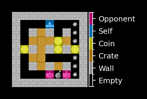
A more effective approach is one-hot encoding. Instead of compressing all cell types into a single grid of integers, we give each type its own binary layer. For example, one \(9\times9\) array marks where the walls are (1 = wall, 0 = no wall), another marks crates, another marks coins, and so on. Stacking these layers creates a set of “feature maps” that together describe the state of the game. This format is far easier for a neural network to interpret, since it only needs to detect patterns of 0s and 1s within each layer, rather than decode arbitrary categories. Figure 2 illustrates the idea with the encoding that I chose.
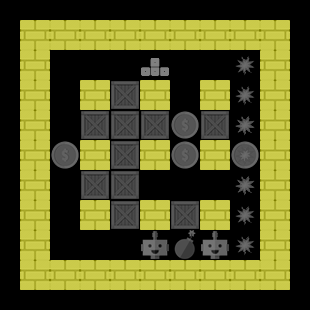
Note that this encoding is not centered on the player. For scaling to larger boards, it often makes sense to center the input around the player and fix the field of view to a certain size (e.g. still 9×9). With this encoding, we could feed the board into fully connected layers, just like in Tic-Tac-Toe. But in practice, this approach is inefficient: the network needs to learn spatial patterns (like corridors, dead-ends, or safe zones) from scratch, and dense layers are not well suited for spatial data. Instead, convolutional layers are a better fit.
You can think of convolutional layers as a collection of small “pattern detectors” that slide across the grid. At first, they recognize local structures such as walls, bombs, or coins in a small neighborhood. When stacked, these detectors combine into larger and more abstract features, such as escape routes or dangerous areas. By the time the output reaches the fully connected layers, the network has already distilled the raw input into (hopefully) meaningful high-level features.
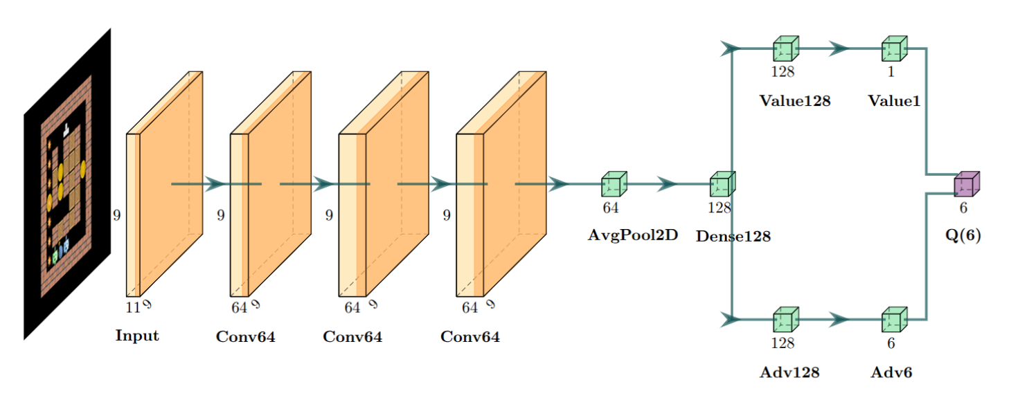
Figure 3 illustrates the neural network architecture I use in the following. The model is built from a stack of convolutional layers, followed by a pooling layer and a duelling head with fully connected layers. The pooling layer averages the spatial output of the last convolutional layer, reducing it to 64 values that serve as high-level features.
I also tried flattening the output of the third convolution directly into a linear array with 64 × 9 × 9 elements. Feeding this into the fully connected layer did work, but it resulted in a layer with over ~600k parameters. The network then showed poor generalisation: it played well against other agents but completely failed in unseen environments such as the coin-heaven scenario (with only coins and no enemies or crates).
Introducing the pooling layer fixed this issue by both improving generalisation and balancing the number of parameters between the convolutional and fully connected layers. Reducing the number of filters in the convolutional layers led to worse performance, so I consider 64 filters the minimum required for this task.
The training process
Most hyperparameters & rewards are unchanged compared to the last post. For reference, the unchanged parameters are:
- Coins: 1 point per coin
- Kills: 5 points per enemy killed
- Crate density: Default is
0.75, can be adjusted by scenario - Number of coins: Default is
9, can be adjusted by scenario - Board size: My default is
9x9(including walls) - Bombs: Explode in the
4th frame after being dropped, explosion affects a radius of3fields and is present for2frames - Discount factor (γ): 0.8
- Max steps: 400
I also left the reward system unchanged:
| Event | Reward | Description |
|---|---|---|
| COIN_COLLECTED | +0.20 | Agent collected a coin |
| KILLED_OPPONENT | +1.00 | Agent killed another agent |
| CRATE_DESTROYED | +0.10 | Agent destroyed a crate |
| BOMB_DROPPED | +0.02 | Agent dropped a bomb |
| KILLED_SELF | −0.90 | Agent killed itself |
| GOT_KILLED | −1.00 | Agent got killed by opponent |
| WAITED | −0.02 | Agent performed a WAIT action |
| INVALID_ACTION | −0.02 | Agent performed an invalid action |
Note that the value of KILLED_SELF should ideally be slightly positive. In the case of suicide, the agent receives both the GOT_KILLED and KILLED_SELF rewards. Since suicide is preferable to being killed by an opponent - because no one else scores points-it makes sense to reflect that in the reward structure. However, simplifying the reward scheme actually degraded performance. I found it important to strongly incentivise the agent to drop bombs and destroy crates.
I used the following hyperparameters specific to DQN:
- Learning rate (α): 3e-4. Higher rates led to instability, while lower ones slowed training.
- Batch size: 64. I did not experiment with different batch sizes, but for training with a GPU higher batch sizes will probably lead to higher performance.
- Gradient steps: 4. This means four gradient updates per training update. With up to 400 transitions per game episode, we insert 400 transitions into the buffer but only train on 4 × 64 = 256 samples. As a result, each transition is visited at most once, making the replay buffer almost ineffective. I plan to address this in a follow-up post.
- Exploration: ε decays from 1 to 0.1 with a per-episode decay factor of 0.999. After ~1,000 episodes, ε is around 0.3, and it reaches 0.1 after ~3,000 episodes.
- Prioritised experience replay: Training starts once the buffer contains 10,000 transitions (roughly 1,000 episodes). The buffer capacity is 100,000 transitions (about 250 full episodes). I anneal toward unbiased updates over 100,000 gradient steps (~25,000 episodes).
- Double DQN: The target network is updated with a hard copy of the online network every 10 gradient updates. Larger intervals, such as 30, also worked well in my experiments.
Bombs are all that counts
I simulate a full game in the classic scenario with multiple agents:
- A rule-based agent
- A rule-based agent based on the simplified state representation from the tabular Q-learning post (the representator)
- A peaceful agent that moves randomly and never places bombs
- A Deep Q-learning agent (cnn_allstar)
Training was run for 100,000 episodes. On my laptop CPU, this translated to about 2–4 episodes per second, meaning several hours of runtime. I suspect there are still performance bottlenecks in the code, but a quick flame graph analysis didn’t reveal anything obvious. A large fraction of computation time is spent in convolutional and fully connected layer updates, specifically matrix multiplications.
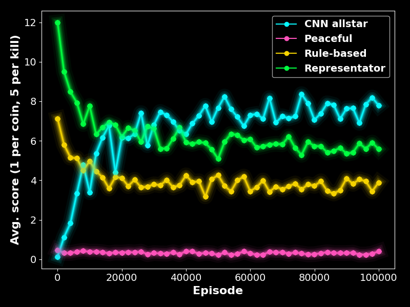
Running on a GPU did not noticeably accelerate training, likely because communication overhead dominates execution time for a network of this size (~0.5 MB). After 100,000 training episodes, the cnn_allstar plays reasonably well, often achieving higher scores than both the rule-based agent and the representator.
Next, we assess the performance of the cnn_allstar by studying the averaged results of 1,000 games between the cnn_allstar agent, a rule-based agent, the tabular-Q allstar agent (allstar) from the previous post and the representator.
| Category | cnn_allstar | rule-based agent | allstar | representator |
|---|---|---|---|---|
| bombs | 35 | 6.9 | 11 | 13 |
| coins | 2.7 | 1.5 | 2.6 | 2.2 |
| crates | 6.1 | 4.6 | 4.4 | 5.8 |
| invalid | 1.9 | 4.7 | 1.6 | 3.4 |
| kills | 0.55 | 0.17 | 0.21 | 0.28 |
| moves | 2.1e+02 | 90 | 1.2e+02 | 1.3e+02 |
| score | 5.4 | 2.4 | 3.6 | 3.6 |
| steps | 2.6e+02 | 1.1e+02 | 1.4e+02 | 1.5e+02 |
| suicides | 0.26 | 0.37 | 0.52 | 0.47 |
| time | 0.39 | 0.065 | 0.093 | 0.077 |
Overall, the cnn_allstar agent places more bombs and is a stronger killer than the built-in rule-based agent, the representator, and the allstar. It consistently achieves higher scores than the other agents while committing fewer suicides.
The training process is shown in Figure 5. Without the duelling head - when feeding the one-hot encoding directly into fully connected layers - the DQN agent’s performance plateaued at an average score of about 4. Flattening the convolutional output without pooling allowed the cnn_allstar to occasionally reach scores around 8, but training stability was generally poorer.
Extrapolate to the unseen?
One important capability the agent should have, at least in theory, is the ability to extrapolate to unseen situations. The figure below demonstrates that the cnn_allstar, despite never encountering the coin-heaven scenario during training, is sometimes able to collect all coins. This demonstrates that the network architecture does not terribly overfit the training data.
What do the convolutional layers actually see?
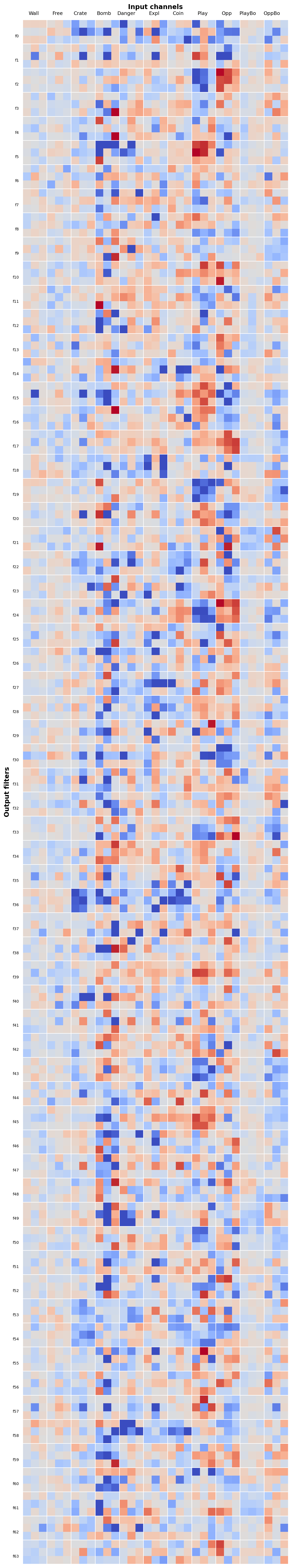
One thing I’ve been curious about is whether we can actually see the high-level features the convolutional layers are pulling out of the one-hot encoded data. As a first step, I plotted the weights of the cnn_allstar’s first convolutional layer’s filters (ignoring biases) after 100,000 episodes of training - shown in Figure 7. The first convolutional layer takes 11 input channels and has 64 filters with 3x3 heads giving a total of 6336 parameters shown here. We can clearly see that the parameters processing crate, bomb, player and opponent channels have the highest magnitudes. We can speculate about the interpretation of some of these filters:
- f0 reacts to a situation where there are wall above and below and the agent can walk left and right when there is an explosion on the left
- f1 reacts to the absence of a wall, crate, bomb and explosion and has a positive activation for a free field and when a player is around and especially left of the free tile
- f2 reacts to opponents that can move to a free field in the absence of a player
To verify this intuition based on the convolutional layer weights, we can instead look at activations. For example, the first convolutional layer maps the 9 × 9 × 11 input into a 9 × 9 × 64 output. Plotting these 64 activation maps side by side and overlaying them with the original game state gives us a sense of what each filter responds to. Figure 8 shows these activation patterns across the layers. Looking at the first filter of the first layer in frame 1, for instance, we can confirm that the activation indicates a free field to the right the player can move to. Please feel free to explore them in case of interest. But in general, I still find the results hard to interpret. Please reach out to me if there are better ways to visualise and understand CNN activations.
Conclusion
In this post, we trained a DQN algorithm with a convolutional neural network to play a Bomberman clone. The approach proved effective: the final agent outperformed the tabular Q-agent developed earlier, and it did so without heavy reliance on handcrafted features. Training this agent was more complex than training the tabular Q-agent, but in my view the solution is far more elegant.
Looking ahead, I’d like to refine the state encoding - for example, by stacking multiple frames to provide temporal context - and also explore how well the agent can learn directly from raw RGB image input.